5.2. Example 2 - Longslit large-dither point source - using the “reduce” command line
In this example, we will reduce a GMOS longslit observation of ORC J0102-2450, an Odd Radio Circle, using the “reduce” command that is operated directly from the unix shell. Just open a terminal and load the DRAGONS conda environment to get started.
This observation dithers along the dispersion axis by several tens of nanometer.
5.2.1. The dataset
If you have not already, download and unpack the tutorial’s data package. Refer to Downloading tutorial datasets for the links and simple instructions.
The dataset specific to this example is described in:
Here is a copy of the table for quick reference.
Science |
S20220611S0717 (705 nm)
S20220611S0716 (795 nm)
|
Science biases |
S20220610S0182-186
S20220611S0827,829,830,832,834
|
Science flats |
S20220611S0718 (705 nm)
S20220611S0715 (795 nm)
|
Science arcs |
S20220611S0782 (705 nm)
S20220611S0779 (795 nm)
|
Standard (LTT7379) |
S20220608S0098 (705 nm)
S20220608S0101 (795 nm)
|
Standard biases |
S20220608S0186-190
S20220609S0206-210
|
Standard flats |
S20220608S0099 (705 nm)
S20220608S0100 (795 nm)
|
Standard arc |
S20220608S0124 (705 nm)
S20220608S0125 (795 nm)
|
BPM |
bpm_20220128_gmos-s_Ham_22_full_12amp.fits
|
5.2.2. Configuring the interactive interface
In ~/.dragons/, add the following to the configuration file dragonsrc:
[interactive]
browser = your_prefered_browser
The [interactive] section defines your prefered browser. DRAGONS will open
the interactive tools using that browser. The allowed strings are “safari”,
“chrome”, and “firefox”.
5.2.3. Set up the Local Calibration Manager
Important
Remember to set up the calibration service.
Instructions to configure and use the calibration service are found in Setting up the Calibration Service, specifically these sections: The Configuration File and Usage from the Command Line.
5.2.4. Create file lists
This dataset contains science and calibration frames. For some programs, it could contain different observed targets and different exposure times depending on how you like to organize your raw data.
The DRAGONS data reduction pipeline does not organize the data for you. You have to do it. However, DRAGONS provides tools to help you with that.
The first step is to create input file lists. The tool “dataselect” helps with that. It uses Astrodata tags and “descriptors” to select the files and send the filenames to a text file that can then be fed to “reduce”. (See the Astrodata User Manual for information about Astrodata.)
First, navigate to the playground directory in the unpacked data package:
cd <path>/gmosls_tutorial/playground
5.2.4.1. Two lists for the biases
The science observations and the spectrophotometric standard observations were obtained using different regions-of-interest (ROI). So we will need two master biases, one “Full Frame” for the science and one “Central Spectrum” for the standard.
We can use dataselect to select biases for each ROI.
Given the data that we have in the playdata/example2 directory, we can create
our GMOS-S bias list using the tags and an expression that uses the ROI
settings. Remember, this will always depend on what you have in your raw data
directory. For easier selection criteria, you might want to keep raw data
from different programs in different directories.
First, let’s see which biases we have for the different ROIs in our raw data directory.
dataselect ../playdata/example2/*.fits --tags BIAS | showd -d detector_roi_setting

---------------------------------------------------------------
filename                                   detector_roi_setting
---------------------------------------------------------------
../playdata/example2/S20220608S0186.fits       Central Spectrum
../playdata/example2/S20220608S0187.fits       Central Spectrum
../playdata/example2/S20220608S0188.fits       Central Spectrum
../playdata/example2/S20220608S0189.fits       Central Spectrum
../playdata/example2/S20220608S0190.fits       Central Spectrum
../playdata/example2/S20220609S0206.fits       Central Spectrum
../playdata/example2/S20220609S0207.fits       Central Spectrum
../playdata/example2/S20220609S0208.fits       Central Spectrum
../playdata/example2/S20220609S0209.fits       Central Spectrum
../playdata/example2/S20220609S0210.fits       Central Spectrum
../playdata/example2/S20220610S0182.fits             Full Frame
../playdata/example2/S20220610S0183.fits             Full Frame
../playdata/example2/S20220610S0184.fits             Full Frame
../playdata/example2/S20220610S0185.fits             Full Frame
../playdata/example2/S20220610S0186.fits             Full Frame
../playdata/example2/S20220611S0827.fits             Full Frame
../playdata/example2/S20220611S0829.fits             Full Frame
../playdata/example2/S20220611S0830.fits             Full Frame
../playdata/example2/S20220611S0832.fits             Full Frame
../playdata/example2/S20220611S0834.fits             Full Frame
We can see the two groups that differ on their ROI. We can use that as a search criterion for creating the list with dataselect
dataselect ../playdata/example2/*.fits --tags BIAS --expr='detector_roi_setting=="Central Spectrum"' -o biasesstd.lis
dataselect ../playdata/example2/*.fits --tags BIAS --expr='detector_roi_setting=="Full Frame"' -o biasessci.lis
5.2.4.2. A list for the flats
The GMOS longslit flats are not normally stacked. The default recipe does not stack the flats. This allows us to use only one list of the flats. Each will be reduced individually, never interacting with the others.
If you have multiple programs and you want to reduce only the flats for that
program, you might want to use the program_id descriptor in the --expr
expression.
Here, we have only one set of flats, so we will just gather them all together.
dataselect ../playdata/example2/*.fits --tags FLAT -o flats.lis
5.2.4.3. A list for the arcs
The GMOS longslit arcs are not normally stacked. The default recipe does not stack the arcs. This allows us to use only one list of arcs. Each will be reduced individually, never interacting with the others.
The arcs normally share the program_id with the science observations, if
you find that you need more accurate sorting. We do not need it here.
dataselect ../playdata/example2/*.fits --tags ARC -o arcs.lis
5.2.4.4. Two lists for the spectrophotometric standard star
If a spectrophotometric standard is recognized as such by DRAGONS, it will
receive the Astrodata tag STANDARD. All spectrophotometric standards
normally used at Gemini are in the DRAGONS list of recognized standards.
For this example, we will be reducing the standard star observations at each
central wavelength separately without stacking them. The standard star reduction
recipe stacks all the observations in a given file list. So we need to create
separate file lists for the different central wavelengths.
First, let’s check the central wavelength of the standard star frames in our raw data directory.
dataselect ../playdata/example2/*.fits --tags STANDARD | showd -d central_wavelength

-------------------------------------------------------------
filename                                   central_wavelength
-------------------------------------------------------------
../playdata/example2/S20220608S0098.fits             7.05e-07
../playdata/example2/S20220608S0101.fits             7.95e-07
We will then create two standard star lists for the two central wavelengths.
dataselect ../playdata/example2/*.fits --tags STANDARD --expr='central_wavelength==7.05e-07' -o std_705nm.lis
dataselect ../playdata/example2/*.fits --tags STANDARD --expr='central_wavelength==7.95e-07' -o std_795nm.lis
5.2.4.5. A list for the science observations
The science observations are what is left, that is anything that is not a
calibration. Calibrations are assigned the astrodata tag CAL, therefore
we can select against that tag to get the science observations.
If we had multiple targets, we would need to split them into separate list. To inspect what we have we can use dataselect and showd together.
dataselect ../playdata/example2/*.fits --xtags CAL | showd -d object

-------------------------------------------------
filename                                   object
-------------------------------------------------
../playdata/example2/S20220611S0716.fits     ORC5
../playdata/example2/S20220611S0717.fits     ORC5
Here we only have one object from the same sequence. We would not need any expression, just excluding calibrations would be sufficient. But we demonstrate here how one would specify the object name for a more surgical selection.
dataselect ../playdata/example2/*.fits --xtags CAL --expr='object=="ORC5"' -o sci.lis
5.2.5. Bad Pixel Mask
Starting with DRAGONS v3.1, the bad pixel masks (BPMs) are now handled as calibrations. They are downloadable from the archive instead of being packaged with the software. They are automatically associated like any other calibrations. This means that the user now must download the BPMs along with the other calibrations and add the BPMs to the local calibration manager.
See Getting Bad Pixel Masks from the archive in Tips and Tricks to learn about the various ways to get the BPMs from the archive.
To add the static BPM included in the data package to the local calibration database:
caldb add ../playdata/example2/bpm*.fits
5.2.6. Master Bias
We create the master biases with the “reduce” command. Because the database
was given the “store” option in the dragonsrc file, the processed biases
will be automatically added
to the database at the end of the recipe.
reduce @biasesstd.lis
reduce @biasessci.lis
The master biases are S20220608S0186_bias.fits and S20220610S0182_bias.fits;
this information is in both the terminal log and the log file. The @ character
before the name of the input file is the “at-file” syntax. More details can be found in
the "at-file" Facility documentation.
Note
The file name of the output processed bias is the file name of the
first file in the list with _bias appended as a suffix. This is the
general naming scheme used by “reduce”.
Note
If you wish to inspect the processed calibrations before adding them
to the calibration database, remove the “store” option attached to the
database in the dragonsrc configuration file. You will then have to
add the calibrations manually following your inspection, eg.
caldb add *_bias.fits
5.2.7. Master Flat Field
GMOS longslit flat fields are normally obtained at night along with the observation sequence to match the telescope and instrument flexure. The matching flat nearest in time to the target observation is used to flat field the target. The central wavelength, filter, grating, binning, gain, and read speed must match.
Because of the flexure, GMOS longslit flat fields are not stacked. Each is reduced and used individually. The default recipe takes that into account.
We can send all the flats, regardless of characteristics, to reduce and each will be reduced individually. When a calibration is needed, in this case, a master bias, the best match will be obtained automatically from the local calibration manager.
reduce @flats.lis
The primitive normalizeFlat, used in the recipe, has an interactive mode.
To activate the interactive mode:
reduce @flats.lis -p interactive=True
The interactive tools are introduced in section Interactive tools.
5.2.8. Processed Arc - Wavelength Solution
GMOS longslit arc can be obtained at night with the observation sequence, if requested by the program, but are often obtained at the end of the night or the following afternoon instead. In this example, the arcs have been obtained at night, as part of the sequence. Like the spectroscopic flats, they are not stacked, which means that they can be sent to reduce all together and will be reduced individually.
The wavelength solution is automatically calculated and has been found to be
quite reliable. There might be cases where it fails; inspect the RMS of
determineWavelengthSolution in the logs to confirm a good solution.
reduce @arcs.lis
The primitive determineWavelengthSolution, used in the recipe, has an
interactive mode. To activate the interactive mode:
reduce @arcs.lis -p interactive=True
The interactive tools are introduced in section Interactive tools.
5.2.9. Processed Standard - Sensitivity Function
The GMOS longslit spectrophotometric standards are normally taken when there is a hole in the queue schedule, often when the weather is not good enough for science observations. For a large wavelength dither, i.e., a difference in central wavelength much greater than about 10 nm, a spectrophotometric standard should be taken at each of those positions to calculate the respective sensitvity functions. The latter will then be used for spectrophotometric calibration of the science observations at the corresponding central wavelengths.
The reduction of the standard will be using a BPM, a master bias, a master flat,
and a processed arc. If those have been added to the local calibration
manager, they will be picked up automatically. The output of the reduction
includes the sensitivity function and will be added to the calibration
database automatically if the “store” option is set in the dragonsrc
configuration file.
The 705nm Standard
In most situation, the default recipe and input parameters will yield a good calculation of the sensitivity function.
reduce @std_705nm.lis
However, if you suspect a suboptimal reduction or just want to confirm that
things are going well, there are four primitives in the default recipe for
spectrophotometric standard have an interactive interface:
skyCorrectFromSlit, findApertures,
traceApertures, and calculateSensitivity. To activate the
interactive mode for all four:
reduce @std_705nm.lis -p interactive=True
Since the standard star spectrum is bright and strong, and the exposure short, it is somewhat unlikely that interactivity will be needed for the sky subtraction, or finding and tracing the spectrum. The fitting of the sensitivity function however can sometimes benefit from little adjustment.
To activate the interactive mode only for the measurement of the sensitivity function:
reduce @std_705nm.lis -p calculateSensitivity:interactive=True
The interactive tools are introduced in section Interactive tools.
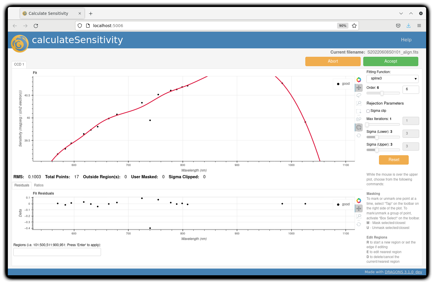
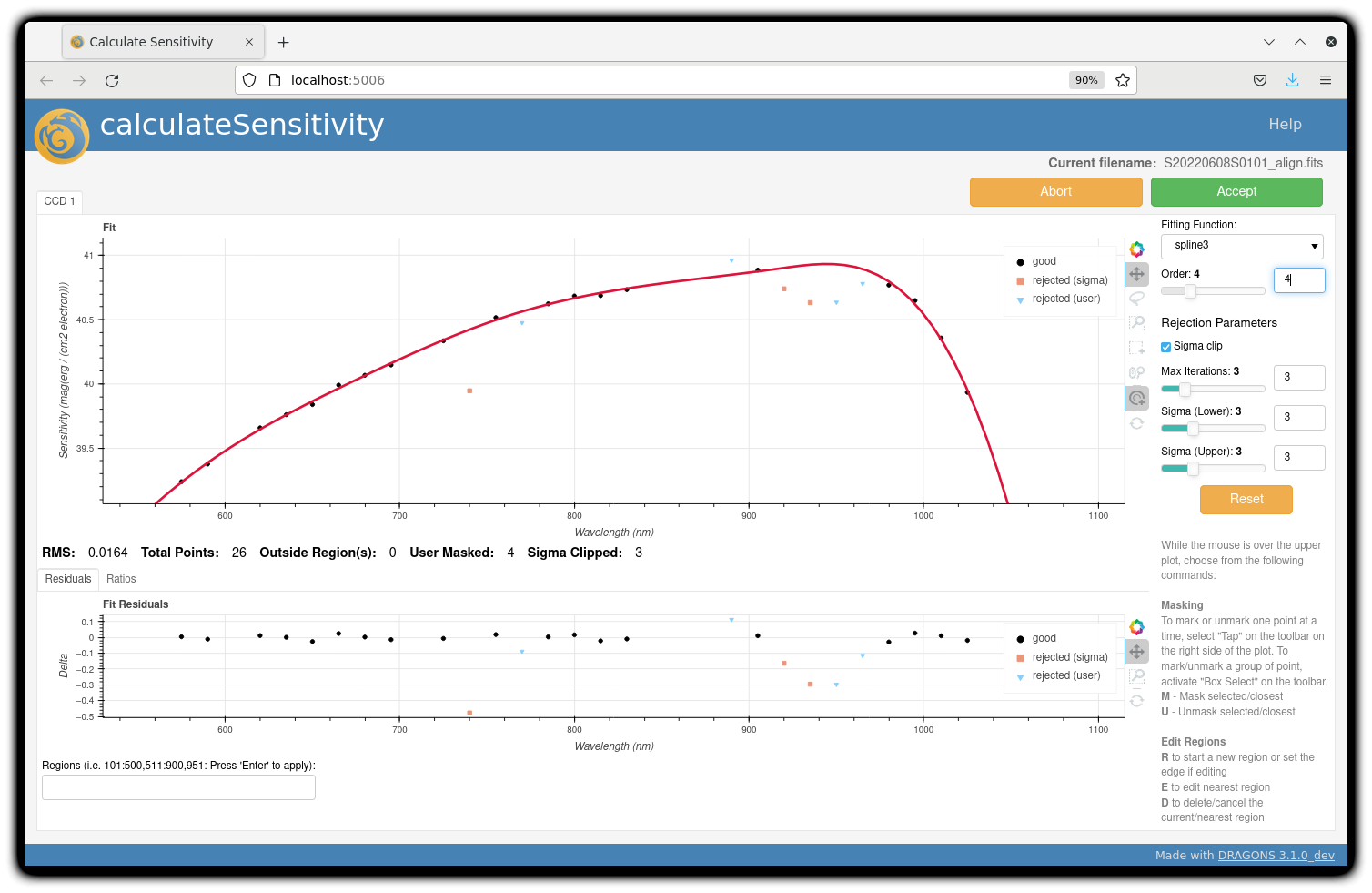
The 795nm Standard
For the standard star observation at central wavelength 795 nm in this
dataset, calculateSensitivity with its default parameter values yields a suboptimal number
of data points to constrain its sensitivity curve (see the left plot below; click the panel to enlarge).
There is a conspicuous gap between 820 and 880 nm – a result of the amplifier #5 issue and compounded
by the presence of telluric absorption redward of around 930 nm.
To deal with this, we can consider interpolating the (reference) data of the spectrophotometric standard,
given that it has a smooth spectrum,
to generate new sensitivity data points to fit.
This is enabled by the resampling parameter, whose value
we update as follows
reduce @std_795nm.lis -p calculateSensitivity:interactive=True calculateSensitivity:resampling=15.0
The resulting curve is shown on the right plot (click the panel to enlarge). Notice that we have manually masked three data points.
Note
If you wish to inspect the spectra:
dgsplot --bokeh S20220608S0098_standard.fits 1
dgsplot --bokeh S20220608S0101_standard.fits 1
where 1 is the aperture #1, the brightest target.
To learn how to plot a 1-D spectrum with matplotlib using the WCS from a
Python script, see Tips and Tricks Plot a 1-D spectrum.
The sensitivity function is stored within the processed standard spectrum. To learn how to plot it, see Tips and Tricks Inspect the sensitivity function.
5.2.10. Science Observations
As mentioned previously, the science target is the central galaxy of an Odd Radio Circle. The sequence has two images that were dithered in wavelength (with a large step of 90 nm). DRAGONS will register the two images, align and stack them before extracting the 1-D spectrum.
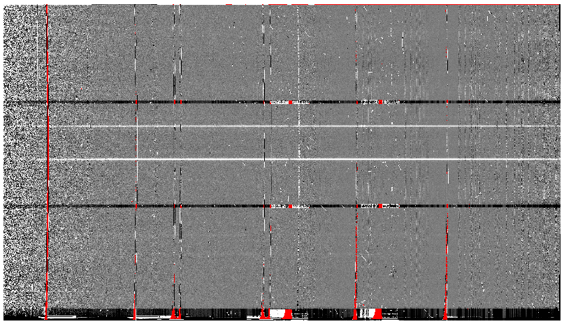
This is what one raw image looks like.
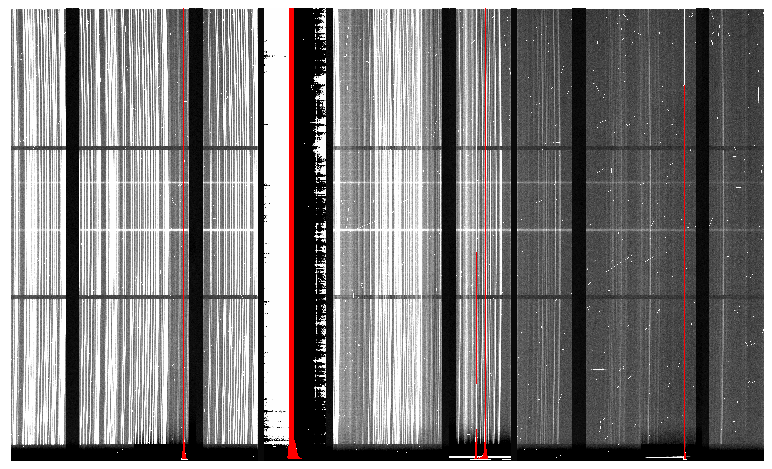
The broad, white and black vertical bands (slightly to the left of the middle) are related to the GMOS-S amplifier #5 issues. As can be seen, there are two obvious sources in this observation. Regardless of whether both of them are of interest to the program, DRAGONS will locate, trace, and extract them automatically. Each extracted spectrum is stored in an individual extension in the output multi-extension FITS file.
With the master bias, the master flat, the processed arcs (one for each of the grating position, aka central wavelength), and the processed standards in the local calibration manager, one only needs to do as follows to reduce the science observations and extract the 1-D spectrum.
reduce -r reduceWithMultipleStandards @sci.lis -p interactive=True
Here we use a different science reduction recipe reduceWithMultipleStandards
than the default. The
default recipe performs flux calibration after stacking the extracted spectra
as described here, which is not suitable
for these observations with a large wavelength dither. The recipe
reduceWithMultipleStandards will run flux calibration for each
central wavelength using the corresponding sensitivity function from the
spectrophotometric standard before stacking
the observations – the desired workflow for this example.
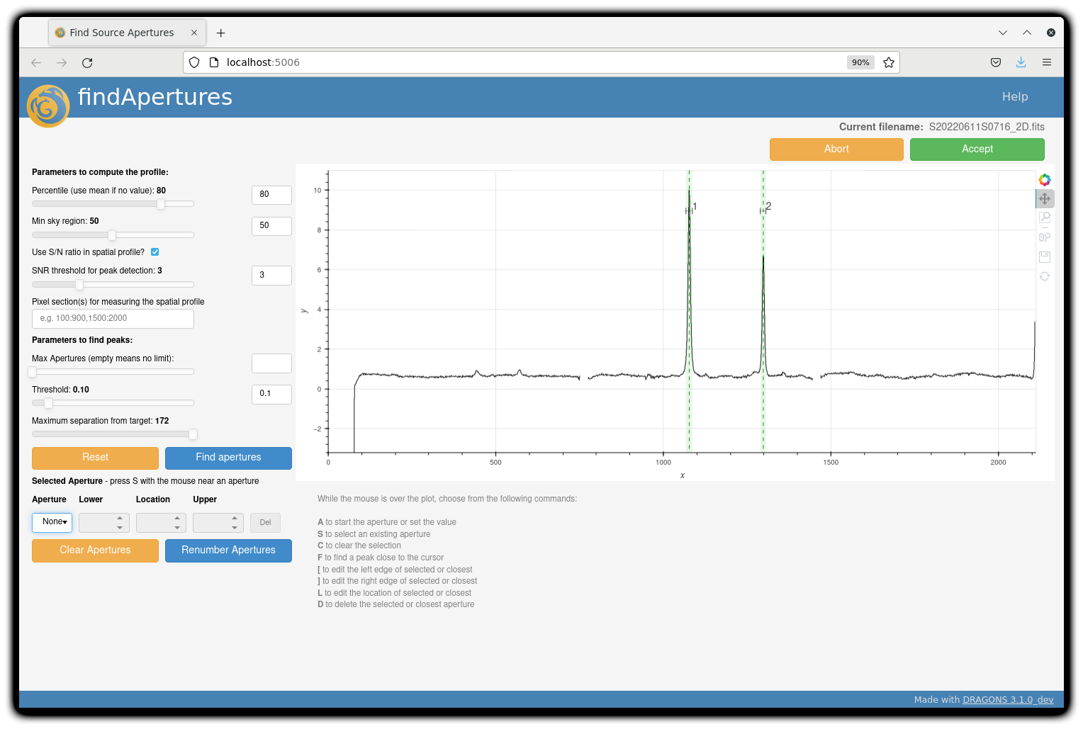
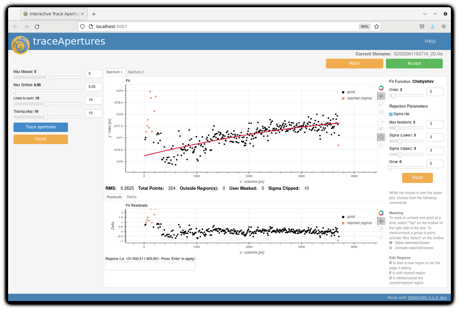
You can make use of the interactive tools to optimize the reduction. For the science reduction above, we have deleted any additional apertures found by DRAGONS barring the two most prominent ones (see the left plot; click to enlarge). You simply hover over the unwanted peak and press D. Furthermore, we have selected sigma-clipping while tracing the apertures (right plot; click to enlarge). Notice that there is an additional tab for Aperture 2 in the upper part of the right plot.
The plots below are from the second findApertures call, the one done on
the stacked image and after the skySubtractFromSlit primitive.
The outputs include a 2-D spectrum image (S20220611S0716_2D.fits), which has been
bias corrected, flat fielded, QE-corrected, wavelength-calibrated, corrected for
distortion, sky-subtracted, flux-calibrated, and stacked, and also the 1-D spectra
(S20220611S0716_1D.fits) extracted from this 2-D spectrum image. The 1-D spectra are stored
as 1-D FITS images in extensions of the output Multi-Extension FITS file, along with their
respective variance and data quality (or mask) arrays.
This is what the 2-D spectrum looks like.
reduce -r display S20220611S0716_2D.fits
Note
ds9 must be launched by the user ahead of running the display primitive.
(ds9& on the terminal prompt.)
The apertures found are listed in the log for the findApertures primitive,
just before the call to traceApertures. Information about the apertures
are also available in the header of each extracted spectrum: XTRACTED,
XTRACTLO, XTRACTHI, for aperture center, lower limit, and upper limit,
respectively.
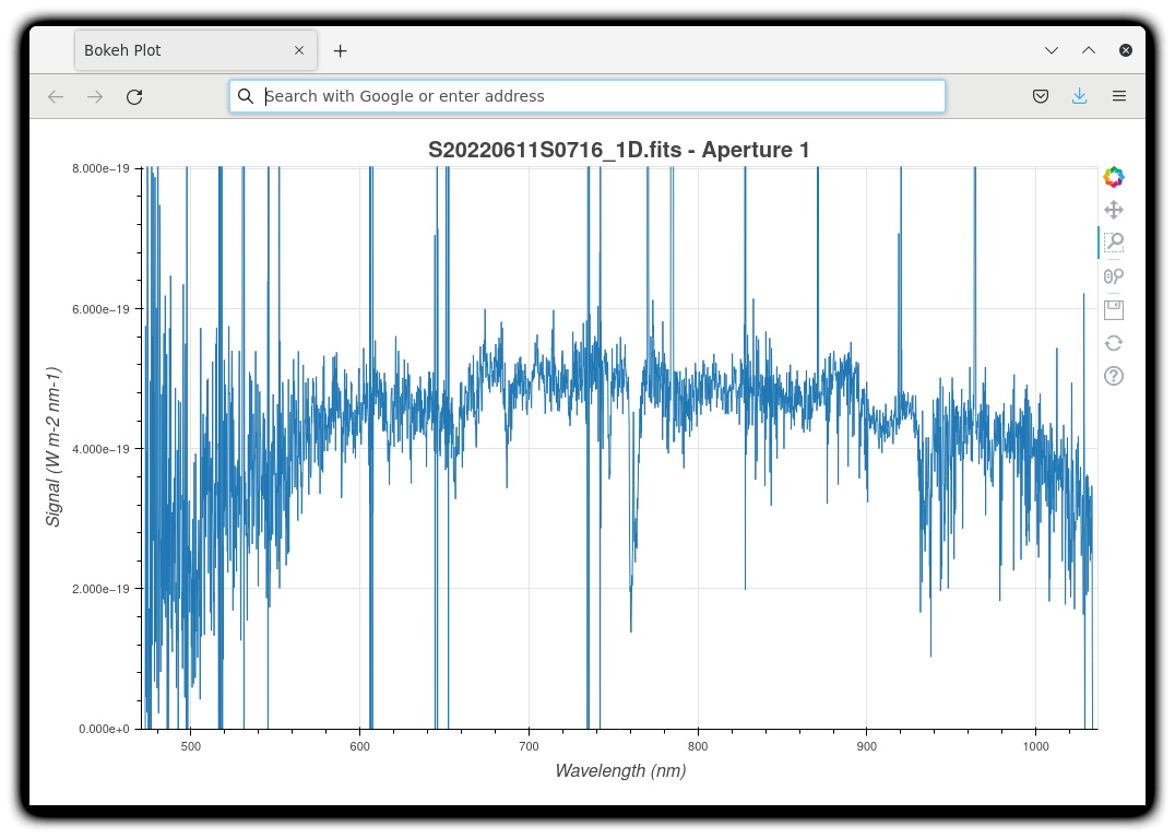
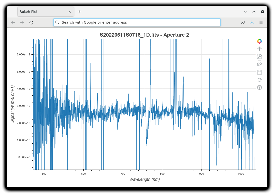
The 1-D flux-calibrated spectra of the two apertures are shown below.
Note
The drop beyond 960nm is related to the lack of coverage in the sensitivity function.
dgsplot --bokeh S20220611S0716_1D.fits 1
dgsplot --bokeh S20220611S0716_1D.fits 2
Since there are only two images, several bad columns, and artifacts remain
in the data. Many are flagged in the mask, the DQ plane of the output FITS
files. Flagged pixels are not used in the calculations. dgsplot
automatically ignore those bad pixels.
If you are using your own tools and they cannot use the DQ plane or mask, you might want to interpolate over the bad values. This is a cosmetic step left to the user as the only purpose is to improve the look of the spectra, not the scientific result.
If you decide to apply a cosmetic correction, you could use the primitive
applyDQPlane (reduce -r applyDQPlane S20220611S0716_1D). We do not
recommend that you do science measurements on a file altered for cosmetic
purposes.
To learn how to plot a 1-D spectrum with matplotlib using the WCS from a Python script, see Tips and Tricks Plot a 1-D spectrum.
If you need an ascii representation of the spectra, you can use the primitive
write1DSpectra to extract the values from the FITS file.
reduce -r write1DSpectra S20220611S0716_1D.fits
The primitive outputs in the various formats offered by astropy.Table. To
see the list, use showpars.
showpars S20220611S0716_1D.fits write1DSpectra
To use a different format, set the format parameters.
reduce -r write1DSpectra -p format=ascii.ecsv extension='ecsv' S20220611S0716_1D.fits