8. Tips and Tricks

8.1. Getting Bad Pixel Masks from the archive

Starting with DRAGONS v3.1, the static bad pixel masks (BPMs) are now handled as calibrations. They are downloadable from the archive instead of being packaged with the software. There are various ways to get the BPMs.

Note that at this time there no static BPMs for Flamingos-2 data.

8.1.1. Manual search

Ideally, the BPMs will show up in the list of associated calibrations, the “Load Associated Calibration” tab on the archive search form (next section). This will happen of all new data. For old data, until we fix an issue recently discovered, they will not show up as associated calibration. But they are there and can easily be found.

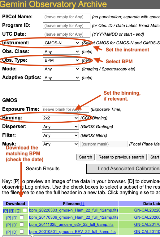
On the archive search form, set the “Instrument” to match your data, set the “Obs.Type” to “BPM”, if relevant for the instrument, set the “Binning”. Hit “Search” and the list of BPMs will show up as illustrated in the figure below.

The date in the BPM file name is a “Valid-from” date. It is valid for data taken on or after that date. Find the one most recent BPM that is valid for your date and download (click on “D”) it. Then follow the instructions found in the tutorial examples.

8.1.2. Associated calibrations

The BPMs are now handled like other calibrations. This means that they are also downloaded from the archive. From the archive search form, once you have identified your science data, select the “Load Associated Calibrations” (which turns to “View Calibrations” once the table is loaded). The BPM will show up with the green background.

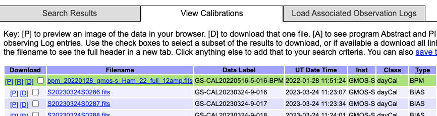
If a BPM does not show up, see if you find one using the manual search explained in the previous section, Manual search.

8.2. Plot a 1-D spectrum

Here is how to plot an extracted spectrum produced by DRAGONS with Python and matplotlib.

import matplotlib.pyplot as plt
import numpy as np

import astrodata
import gemini_instruments

ad = astrodata.open('S20171022S0087_1D.fits')
ad.info()

data = ad[0].data
wavelength = ad[0].wcs(np.arange(data.size)).astype(np.float32)
units = ad[0].wcs.output_frame.unit[0]

# add aperture number and location in the title.
# check that plt.xlabel call.  Not sure it's right, it works though.
plt.xlabel(f'Wavelength ({units})')
plt.ylabel(f'Signal ({ad[0].hdr["BUNIT"]})')
plt.plot(wavelength, data)
plt.show()

8.3. Inspect the sensitivity function

Plotting the sensitivity function is not obvious. Using Python, here’s a way to do it.

import numpy as np
import matplotlib.pyplot as plt

import astrodata
import gemini_instruments
from gempy.library import astromodels as am

ad = astrodata.open('S20170826S0160_standard.fits')

sensfunc = am.table_to_model(ad[0].SENSFUNC)

w = ad[0].wcs(np.arange(ad[0].data.size))

std_wave_unit = ad[0].SENSFUNC['knots'].unit
std_flux_unit = ad[0].SENSFUNC['coefficients'].unit

plt.xlabel(f'Wavelength ({std_wave_unit})')
plt.ylabel(f'{std_flux_unit}')
plt.plot(w, sensfunc(w))
plt.show()

8.4. Useful parameters

8.4.1. skip_primitive

I might happen that you will want or need to not run a primitive in a recipe. You could copy the recipe over and edit it. Or you could invoke the skip_primitive parameter to tell DRAGONS to completely skip that step.

Let’s say that you want the data aligned but not stacked. You would do:

reduce @sci.lis -p stackFrames:skip_primitive=True

8.4.2. write_outputs

When debugging or when there’s a need to inspect intermediate products, you might want to write the output of a specific primitive to disk. This is done with the write_outputs parameter.

For example, to write the extracted spectrum before it is flux calibrated, you would do:

reduce @sci.lis -p extractSpectra:write_outputs=True