4.2. Example 1 - Longslit Dithered Point Source - Using the “reduce” command line
In this example we will reduce a GMOS longslit observation of a DB white dwarf candidate using the “reduce” command that is operated directly from the unix shell. Just open a terminal and load the DRAGONS conda environment to get started.
This observation dithers along the slit and along the dispersion axis.
4.2.1. The dataset
If you have not already, download and unpack the tutorial’s data package. Refer to Downloading tutorial datasets for the links and simple instructions.
The dataset specific to this example is described in:
Here is a copy of the table for quick reference.
Science |
S20171022S0087,89 (515 nm)
S20171022S0095,97 (530 nm)
|
Science biases |
S20171021S0265-269
S20171023S0032-036
|
Science flats |
S20171022S0088 (515 nm)
S20171022S0096 (530 nm)
|
Science arcs |
S20171022S0092 (515 nm)
S20171022S0099 (530 nm)
|
Standard (LTT2415) |
S20170826S0160 (515 nm)
|
Standard biases |
S20170825S0347-351
S20170826S0224-228
|
Standard flats |
S20170826S0161 (515 nm)
|
Standard arc |
S20170826S0162 (515 nm)
|
BPM |
bpm_20140601_gmos-s_Ham_22_full_12amp.fits
|
4.2.2. Configuring the interactive interface
In ~/.dragons/, add the following to the configuration file dragonsrc:
[interactive]
browser = your_preferred_browser
The [interactive] section defines your preferred browser. DRAGONS will open
the interactive tools using that browser. The allowed strings are “safari”,
“chrome”, and “firefox”.
4.2.3. Set up the Local Calibration Manager
Important
Remember to set up the calibration service.
Instructions to configure and use the calibration service are found in Setting up the Calibration Service, specifically the these sections: The Configuration File and Usage from the Command Line.
4.2.4. Create file lists
This data set contains science and calibration frames. For some programs, it could contain different observed targets and different exposure times depending on how you like to organize your raw data.
The DRAGONS data reduction pipeline does not organize the data for you. You have to do it. However, DRAGONS provides tools to help you with that.
The first step is to create input file lists. The tool “dataselect” helps with that. It uses Astrodata tags and “descriptors” to select the files and send the filenames to a text file that can then be fed to “reduce”. (See the Astrodata User Manual for information about Astrodata.)
First, navigate to the playground directory in the unpacked data package:
cd <path>/gmosls_tutorial/playground
4.2.4.1. Two lists for the biases
The science observations and the spectrophotometric standard observations were obtained using different regions-of-interest (ROI). So we will need two master biases, one “Full Frame” for the science and one “Central Spectrum” for the standard.
We can use dataselect to select biases for each ROIs.
Given the data that we have in the playdata directory, we can create
our GMOS-S bias list using the tags and an expression that uses the ROI
settings. Remember, this will always depend on what you have in your raw data
directory. For easier selection criteria, you might want to keep raw data
from different programs in different directories.
First, let’s see which biases we have for in our raw data directory.
dataselect ../playdata/example1/*.fits --tags BIAS | showd -d detector_roi_setting

-------------------------------------------------------------------
filename                                       detector_roi_setting
-------------------------------------------------------------------
../playdata/example1/S20170825S0347.fits       Central Spectrum
../playdata/example1/S20170825S0348.fits       Central Spectrum
../playdata/example1/S20170825S0349.fits       Central Spectrum
../playdata/example1/S20170825S0350.fits       Central Spectrum
../playdata/example1/S20170825S0351.fits       Central Spectrum
../playdata/example1/S20170826S0224.fits       Central Spectrum
../playdata/example1/S20170826S0225.fits       Central Spectrum
../playdata/example1/S20170826S0226.fits       Central Spectrum
../playdata/example1/S20170826S0227.fits       Central Spectrum
../playdata/example1/S20170826S0228.fits       Central Spectrum
../playdata/example1/S20171021S0265.fits             Full Frame
../playdata/example1/S20171021S0266.fits             Full Frame
../playdata/example1/S20171021S0267.fits             Full Frame
../playdata/example1/S20171021S0268.fits             Full Frame
../playdata/example1/S20171021S0269.fits             Full Frame
../playdata/example1/S20171023S0032.fits             Full Frame
../playdata/example1/S20171023S0033.fits             Full Frame
../playdata/example1/S20171023S0034.fits             Full Frame
../playdata/example1/S20171023S0035.fits             Full Frame
../playdata/example1/S20171023S0036.fits             Full Frame
We can see the two groups that differ on their ROI. We can use that as a search criterion for creating the list with dataselect
dataselect ../playdata/example1/*.fits --tags BIAS --expr='detector_roi_setting=="Central Spectrum"' -o biasesstd.lis
dataselect ../playdata/example1/*.fits --tags BIAS --expr='detector_roi_setting=="Full Frame"' -o biasessci.lis
4.2.4.2. A list for the flats
The GMOS longslit flats are not normally stacked. The default recipe does not stack the flats. This allows us to use only one list of the flats. Each will be reduced individually, never interacting with the others.
If you have multiple programs and you want to reduce only the flats for that
program, you might want to use the program_id descriptor in the --expr
expression.
Here, we have only one set of flats, so we will just gather them all together.
dataselect ../playdata/example1/*.fits --tags FLAT -o flats.lis
4.2.4.3. A list for the arcs
The GMOS longslit arcs are not normally stacked. The default recipe does not stack the arcs. This allows us to use only one list of arcs. Each will be reduced individually, never interacting with the others.
The arcs normally share the program_id with the science observations, if
you find that you need more accurate sorting. We do not need it here.
dataselect ../playdata/example1/*.fits --tags ARC -o arcs.lis
4.2.4.4. A list for the spectrophotometric standard star
If a spectrophotometric standard is recognized as such by DRAGONS, it will
receive the Astrodata tag STANDARD. All spectrophotometric standards
normally used at Gemini are in the DRAGONS list of recognized standards.
dataselect ../playdata/example1/*.fits --tags STANDARD -o std.lis
4.2.4.5. A list for the science observations
The science observations are what is left, that is anything that is not a
calibration. Calibrations are assigned the astrodata tag CAL, therefore
we can select against that tag to get the science observations.
If we had multiple targets, we would need to split them into separate list. To inspect what we have we can use dataselect and showd together.
dataselect ../playdata/example1/*.fits --xtags CAL | showd -d object

-----------------------------------------------------
filename                                       object
-----------------------------------------------------
../playdata/example1/S20171022S0087.fits   J2145+0031
../playdata/example1/S20171022S0089.fits   J2145+0031
../playdata/example1/S20171022S0095.fits   J2145+0031
../playdata/example1/S20171022S0097.fits   J2145+0031
Here we only have one object from the same sequence. We would not need any expression, just excluding calibrations would be sufficient. But we demonstrate here how one would specify the object name for a more surgical selection.
dataselect ../playdata/example1/*.fits --xtags CAL --expr='object=="J2145+0031"' -o sci.lis
4.2.5. Bad Pixel Mask
Starting with DRAGONS v3.1, the bad pixel masks (BPMs) are now handled as calibrations. They are downloadable from the archive instead of being packaged with the software. They are automatically associated like any other calibrations. This means that the user now must download the BPMs along with the other calibrations and add the BPMs to the local calibration manager.
See Getting Bad Pixel Masks from the archive in Tips and Tricks to learn about the various ways to get the BPMs from the archive.
To add the static BPM included in the data package to the local calibration database:
caldb add ../playdata/example1/bpm*.fits
4.2.6. Master Bias
We create the master biases with the “reduce” command. Because the database
was given the “store” option in the dragonsrc file, the processed biases
will be automatically added
to the database at the end of the recipe.
reduce @biasesstd.lis
reduce @biasessci.lis
The master biases are S20170825S0347_bias.fits and S20171021S0265_bias.fits;
this information is in both the terminal log and the log file. The @ character
before the name of the input file is the “at-file” syntax. More details can be found in
the "at-file" Facility documentation.
Note
The file name of the output processed bias is the file name of the
first file in the list with _bias appended as a suffix. This the
general naming scheme used by “reduce”.
Note
If you wish to inspect the processed calibrations before adding them
to the calibration database, remove the “store” option attached to the
database in the dragonsrc configuration file. You will then have to
add the calibrations manually following your inspection, eg.
caldb add *_bias.fits
4.2.7. Master Flat Field
GMOS longslit flat fields are normally obtained at night along with the observation sequence to match the telescope and instrument flexure. The matching flat nearest in time to the target observation is used to flat field the target. The central wavelength, filter, grating, binning, gain, and read speed must match.
Because of the flexure, GMOS longslit flat fields are not stacked. Each is reduced and used individually. The default recipe takes that into account.
We can send all the flats, regardless of characteristics, to reduce and each will be reduce individually. When a calibration is needed, in this case, a master bias, the best match will be obtained automatically from the local calibration manager.
reduce @flats.lis
The primitive normalizeFlat, used in the recipe, has an interactive mode.
To activate the interactive mode:
reduce @flats.lis -p interactive=True
The interactive tools are introduced in section Interactive tools.
4.2.8. Processed Arc - Wavelength Solution
GMOS longslit arc can be obtained at night with the observation sequence, if requested by the program, but are often obtained at the end of the night or the following afternoon instead. In this example, the arcs have been obtained at night, as part of the sequence. Like the spectroscopic flats, they are not stacked which means that they can be sent to reduce all together and will be reduced individually.
The wavelength solution is automatically calculated and has been found to be
quite reliable. There might be cases where it fails; inspect the
*_wavelengthSolutionDetermined.pdf plot and the RMS of determineWavelengthSolution in the
logs to confirm a good solution.
reduce @arcs.lis
The primitive determineWavelengthSolution, used in the recipe, has an
interactive mode. To activate the interactive mode:
reduce @arcs.lis -p interactive=True
The interactive tools are introduced in section Interactive tools.
4.2.9. Processed Standard - Sensitivity Function
The GMOS longslit spectrophotometric standards are normally taken when there is a hole in the queue schedule, often when the weather is not good enough for science observations. One standard per configuration, per program is the norm. If you dither along the dispersion axis, most likely only one of the positions will have been used for the spectrophotometric standard. This is normal for baseline calibrations at Gemini. The standard is used to calculate the sensitivity function. It has been shown that a difference of 10 or so nanometers in central wavelength setting does not significantly impact the spectrophotometric calibration.
The reduction of the standard will be using a BPM, a master bias, a master flat,
and a processed arc. If those have been added to the local calibration
manager, they will be picked up automatically. The output of the reduction
includes the sensitivity function and will be added to the calibration
database automatically if the “store” option is set in the dragonsrc
configuration file.
reduce @std.lis
Four primitives in the default recipe for spectrophotometric standard have
an interactive interface: skyCorrectFromSlit, findApertures,
traceApertures, and calculateSensitivity. To activate the interactive
mode for all four:
reduce @std.lis -p interactive=True
Since the standard star spectrum is bright and strong, and the exposure short, it is somewhat unlikely that interactivity will be needed for the sky subtraction, or finding and tracing the spectrum. The fitting of the sensitivity function however can sometimes benefit from little adjustment.
To activate the interactive mode only for the measurement of the sensitivity function:
reduce @std.lis -p calculateSensitivity:interactive=True
Here is an example of what could be adjusted in this particular case. The plots below show the default fit on the left, and the adjusted fit on the right. All that was changed is that the order of the fit was set to “4” instead of the default “6”. You can see how the flaring at the red-end is reduced.
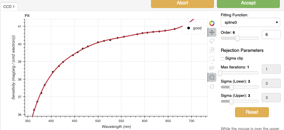
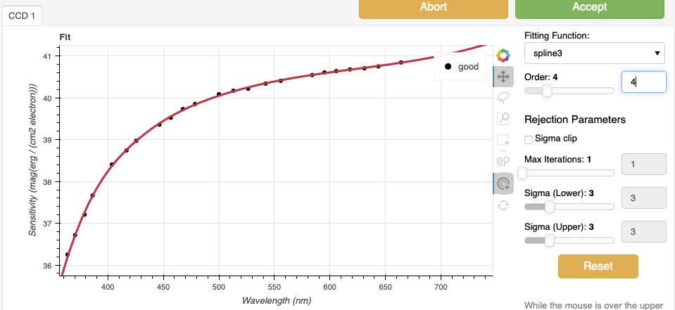
The interactive tools are introduced in section Interactive tools.
Note
If you wish to inspect the spectrum:
dgsplot S20170826S0160_standard.fits 1
where 1 is the aperture #1, the brightest target.
To learn how to plot a 1-D spectrum with matplotlib using the WCS from a
Python script, see Tips and Tricks Plot a 1-D spectrum.
The sensitivity function is stored within the processed standard spectrum. To learn how to plot it, see Tips and Tricks Inspect the sensitivity function.
4.2.10. Science Observations
The science target is a DB white dwarf candidate. The sequence has four images that were dithered spatially and along the dispersion axis. DRAGONS will register the four images in both directions, align and stack them before extracting the 1-D spectrum.
Note
In this observation, there is only one source to extract. If there were multiple sources in the slit, regardless of whether they are of interest to the program, DRAGONS will locate them, trace them, and extract them automatically. Each extracted spectrum is stored in an individual extension in the output multi-extension FITS file.
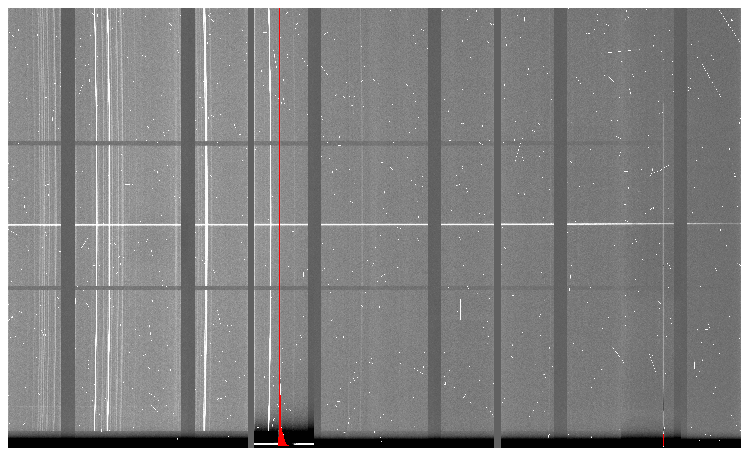
This is what one raw image looks like.
With the master bias, the master flat, the processed arcs (one for each of the grating position, aka central wavelength), and the processed standard in the local calibration manager, one only needs to do as follows to reduce the science observations and extract the 1-D spectrum.
reduce @sci.lis
This produces a 2-D spectrum (S20171022S0087_2D.fits) which has been
bias corrected, flat fielded, QE-corrected, wavelength-calibrated, corrected for
distortion, sky-subtracted, and stacked. It also produces the 1-D spectrum
(S20171022S0087_1D.fits) extracted from that 2-D spectrum. The 1-D
spectrum is flux calibrated with the sensitivity function from the
spectrophotometric standard. The 1-D spectra are stored as 1-D FITS images in
extensions of the output Multi-Extension FITS file.
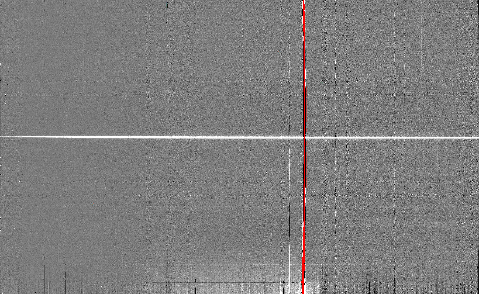
This is what the 2-D spectrum looks like.
reduce -r display S20171022S0087_2D.fits
Note
ds9 must be launched by the user ahead of running the display primitive.
(ds9& on the terminal prompt.)
The apertures found are listed in the log for the findApertures primitive,
just before the call to traceApertures. Information about the apertures
are also available in the header of each extracted spectrum: XTRACTED,
XTRACTLO, XTRACTHI, for aperture center, lower limit, and upper limit,
respectively.
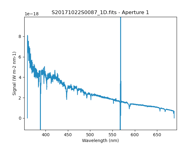
This is what the 1-D flux-calibrated spectrum of our sole target looks like.
Note that any pixels flagged in the data quality array (DQ in the FITS file, or
ad.mask in Python) are not plotted by default. To over-ride that behavior,
dgsplot S20171022S0087_1D.fits 1
To learn how to plot a 1-D spectrum with matplotlib using the WCS from a Python script, see Tips and Tricks Plot a 1-D spectrum.
If you need an ascii representation of the spectum, you can use the primitive
write1DSpectra to extract the values from the FITS file.
reduce -r write1DSpectra S20171022S0087_1D.fits
The primitive outputs in the various formats offered by astropy.Table. To
see the list, use showpars.
showpars S20171022S0087_1D.fits write1DSpectra
To use a different format, set the format parameters.
reduce -r write1DSpectra -p format=ascii.ecsv extension='ecsv' S20171022S0087_1D.fits