7.2. Example 4 - Nod-and-Shuffle Correct for Extra Order - Using the “reduce” command line

In this example we will reduce a GMOS longslit nod-and-shuffle observation of a high redshift quasar. The particularity here is that the setting is quite red and the second order shows up in the spectrum. The configuration uses the OG515 blocking filter and the second order light appears at 1030nm. We will show how to recognize the effect and then how to not include the light from that extra order using the interactive tools.

This observation dithers along the dispersion axis.

7.2.1. The dataset

If you have not already, download and unpack the tutorial’s data package. Refer to Downloading tutorial datasets for the links and simple instructions.

The dataset specific to this example is described in:

Example 4 - Datasets descriptions.

Here is a copy of the table for quick reference.

Science	N20080830S0261 (900 nm) N20080830S0262 (890 nm) N20080830S0265 (880 nm)
Science biases	N20080830S0527-531
Science flats	N20080830S0260 (900 nm) N20080830S0263 (890 nm) N20080830S0264 (880 nm)
Science arcs	N20080830S0491 (900 nm) N20080830S0492 (890 nm) N20080830S0493 (880 nm)
Standard (G191B2B)	N20190902S0046 (900 nm)
Standard biases	N20081011S0313-317
Standard flats	N20081010S0534 (900 nm)
Standard arc	N20081010S0552 (900 nm)
BPM	bpm_20010801_gmos-n_EEV_22_full_3amp.fits

7.2.2. Configuring the interactive interface

In ~/.dragons/, add the following to the configuration file dragonsrc:

[interactive]
browser = your_preferred_browser

The [interactive] section defines your preferred browser. DRAGONS will open the interactive tools using that browser. The allowed strings are “safari”, “chrome”, and “firefox”.

7.2.3. Set up the Local Calibration Manager

Important

Remember to set up the calibration service.

Instructions to configure and use the calibration service are found in Setting up the Calibration Service, specifically the these sections: The Configuration File and Usage from the Command Line.

7.2.4. Create file lists

This data set contains science and calibration frames. For some programs, it could contain different observed targets and different exposure times depending on how you like to organize your raw data.

The DRAGONS data reduction pipeline does not organize the data for you. You have to do it. However, DRAGONS provides tools to help you with that.

The first step is to create input file lists. The tool “dataselect” helps with that. It uses Astrodata tags and “descriptors” to select the files and send the filenames to a text file that can then be fed to “reduce”. (See the Astrodata User Manual for information about Astrodata.)

First, navigate to the playground directory in the unpacked data package:

cd <path>/gmosls_tutorial/playground

7.2.4.1. Two lists for the biases

The science observations and the spectrophotometric standard observations were obtained using different regions-of-interest (ROI). So we will need two master biases, one “Full Frame” for the science and one “Central Spectrum” for the standard.

We can use dataselect to select biases for each ROIs.

Given the data that we have in the playdata directory, we can create our GMOS-N bias list using the tags and an expression that uses the ROI settings. Remember, this will always depend on what you have in your raw data directory. For easier selection criteria, you might want to keep raw data from different programs in different directories.

Let’s see which biases we have for in our raw data directory.

dataselect ../playdata/example4/*.fits --tags BIAS | showd -d detector_roi_setting

---------------------------------------------------------------
filename                                   detector_roi_setting
---------------------------------------------------------------
../playdata/example4/N20080830S0527.fits             Full Frame
../playdata/example4/N20080830S0528.fits             Full Frame
../playdata/example4/N20080830S0529.fits             Full Frame
../playdata/example4/N20080830S0530.fits             Full Frame
../playdata/example4/N20080830S0531.fits             Full Frame
../playdata/example4/N20081011S0313.fits       Central Spectrum
../playdata/example4/N20081011S0314.fits       Central Spectrum
../playdata/example4/N20081011S0315.fits       Central Spectrum
../playdata/example4/N20081011S0316.fits       Central Spectrum
../playdata/example4/N20081011S0317.fits       Central Spectrum

We can see the two groups that differ on their ROI. We can use that as a search criterion for creating the list with dataselect

dataselect ../playdata/example4/*.fits --tags BIAS --expr='detector_roi_setting=="Central Spectrum"' -o biasesstd.lis
dataselect ../playdata/example4/*.fits --tags BIAS --expr='detector_roi_setting=="Full Frame"' -o biasessci.lis

7.2.4.2. A list for the darks

Nod-and-shuffle darks are required for the reduction of nod-and-shuffle observations obtained with the EEV CCDs (this case) and the ee2vv CCDs.

dataselect ../playdata/example4/*.fits --tags DARK -o darks.lis

7.2.4.3. A list for the flats

The GMOS longslit flats are not normally stacked. The default recipe does not stack the flats. This allows us to use only one list of the flats. Each will be reduced individually, never interacting with the others.

The flats used for nod-and-shuffle are normal flats. The DRAGONS recipe will “double” the flat and apply it to each beam.

dataselect ../playdata/example4/*.fits --tags FLAT -o flats.lis

7.2.4.4. A list for the arcs

The GMOS longslit arcs are not normally stacked. The default recipe does not stack the arcs. This allows us to use only one list of arcs. Each will be reduced individually, never interacting with the others.

The arcs normally share the program_id with the science observations, if you find that you need more accurate sorting. We do not need it here.

dataselect ../playdata/example4/*.fits --tags ARC -o arcs.lis

7.2.4.5. A list for the spectrophotometric standard star

If a spectrophotometric standard is recognized as such by DRAGONS, it will receive the Astrodata tag STANDARD. All spectrophotometric standards normally used at Gemini are in the DRAGONS list of recognized standards.

dataselect ../playdata/example4/*.fits --tags STANDARD -o std.lis

7.2.4.6. A list for the science observations

The science observations are what is left, that is anything that is not a calibration. Calibrations are assigned the astrodata tag CAL, therefore we can select against that tag to get the science observations.

If we had multiple targets, we would need to split them into separate list. To inspect what we have we can use dataselect and showd together.

dataselect ../playdata/example4/*.fits --xtags CAL | showd -d object

-------------------------------------------------------
filename                                         object
-------------------------------------------------------
../playdata/example4/N20080830S0261.fits   433819088548
../playdata/example4/N20080830S0262.fits   433819088548
../playdata/example4/N20080830S0265.fits   433819088548

Here we only have one object from the same sequence. We would not need any expression, just excluding calibrations is sufficient.

dataselect ../playdata/example4/*.fits --xtags CAL -o sci.lis

7.2.5. Bad Pixel Mask

Starting with DRAGONS v3.1, the bad pixel masks (BPMs) are now handled as calibrations. They are downloadable from the archive instead of being packaged with the software. They are automatically associated like any other calibrations. This means that the user now must download the BPMs along with the other calibrations and add the BPMs to the local calibration manager.

See Getting Bad Pixel Masks from the archive in Tips and Tricks to learn about the various ways to get the BPMs from the archive.

To add the static BPM included in the data package to the local calibration database:

caldb add ../playdata/example4/bpm*.fits

7.2.6. Master Bias

We create the master biases with the “reduce” command. Because the database was given the “store” option in the dragonsrc file, the processed biases will be automatically added to the database at the end of the recipe.

reduce @biasesstd.lis
reduce @biasessci.lis

The master biases are N20081011S0313_bias.fits and N20080830S0527_bias.fits; this information is in both the terminal log and the log file. The @ character before the name of the input file is the “at-file” syntax. More details can be found in the "at-file" Facility documentation.

Note

The file name of the output processed bias is the file name of the first file in the list with _bias appended as a suffix. This the general naming scheme used by “reduce”.

Note

If you wish to inspect the processed calibrations before adding them to the calibration database, remove the “store” option attached to the database in the dragonsrc configuration file. You will then have to add the calibrations manually following your inspection, eg.

caldb add *_bias.fits

7.2.7. Master Nod-and-Shuffle Dark

The nod-and-shuffle darks normally reproduced the same number of charge shuffling as was done for the science data observation. They are done during the day, when daytime work allows, or at night when the weather is bad. This set was obtained 2 months after the science data.

The darks are stacked together. Here we use the same bias as for the science observation to minimize the amount of data required to download for this tutorial. For a science reduction, it might beneficial to use biases that are contemporary to the darks (ie. from around 2008-10-26).

reduce @darks.lis

7.2.8. Master Flat Field

GMOS longslit flat field are normally obtained at night along with the observation sequence to match the telescope and instrument flexure. The matching flat nearest in time to the target observation is used to flat field the target. The central wavelength, filter, grating, binning, gain, and read speed must match.

Because of the flexure, GMOS longslit flat field are not stacked. Each is reduced and used individually. The default recipe takes that into account.

We can send all the flats, regardless of characteristics, to reduce and each will be reduce individually. When a calibration is needed, in this case, a master bias, the best match will be obtained automatically from the local calibration manager.

reduce @flats.lis

7.2.9. Processed Arc - Wavelength Solution

GMOS longslit arc can be obtained at night with the observation sequence, if requested by the program, but are often obtained at the end of the night or the following afternoon instead. In this example, the arcs have been obtained in the morning. Like the spectroscopic flats, they are not stacked which means that they can be sent to reduce all together and will be reduced individually.

The wavelength solution is automatically calculated and the algorithm has been found to be quite reliable. There might be cases where it fails; inspect the *_mosaic.pdf plot and the RMS of determineWavelengthSolution in the logs to confirm a good solution.

reduce @arcs.lis

7.2.10. Processed Standard - Sensitivity Function

The GMOS longslit spectrophotometric standards are normally taken when there is a hole in the queue schedule, often when the weather is not good enough for science observations. One standard per configuration, per program is the norm. If you dither along the dispersion axis, most likely only one of the positions will have been used for the spectrophotometric standard. This is normal for baseline calibrations at Gemini. The standard is used to calculate the sensitivity function. It has been shown that a difference of 10 or so nanometers in central wavelength setting does not significantly impact the spectrophotometric calibration.

The reduction of the standard will be using a BPM, a master bias, a master flat, and a processed arc. If those have been added to the local calibration manager, they will be picked up automatically. The output of the reduction includes the sensitivity function and will be added to the calibration database automatically if the “store” option is set in the dragonsrc configuration file.

reduce @std.lis -p traceApertures:interactive=True calculateSensitivity:interactive=True

The interactive tools are introduced in a later chapter: Interactive tools. Here we will focus on two of them, the one for the trace and the one for the calculation of the sensitivity function.

In both cases, we will adjust the region to use for the fits. This is done by point the cursor on one edge of the region, typing “r”, moving the cursor to the other edge, and typing “r” again. To adjust the edge of an existing region, use “e” and the cursor, and “e” again to confirm the adjustment. See the summary of keyboard shortcuts at the bottom right of the tool, in gray font.

It is also possible to set regions using the “Regions” textbox below the plots.

traceApertures

Here are the before and after fits. The x-axis is in pixels with the red-end to the left, the blue-end to the right. You can see the sharp discontinuity around pixel 1000. The points to left of the discontinuity are from the second order. The flux from the first order (right of discontinuity) fades away, and the second order takes over.

We want the trace to follow the first order light only. The region in gray is what we need to define. Using just those points, the trace matches the first order light much better.

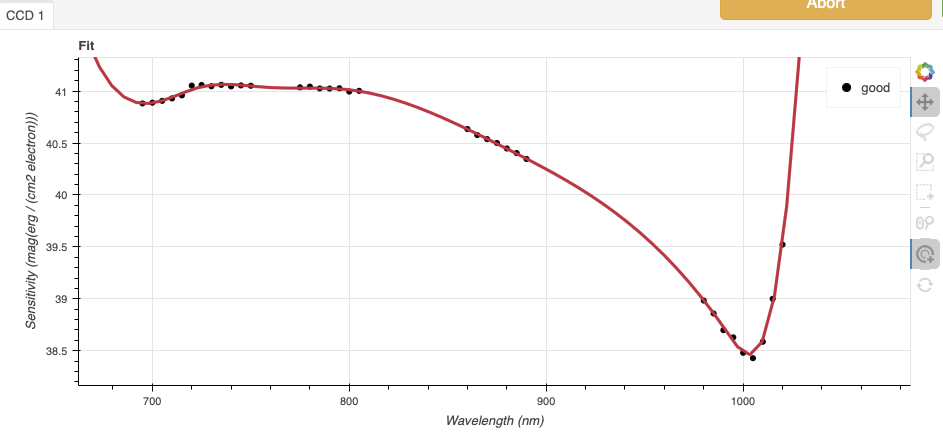
calculateSensitivity

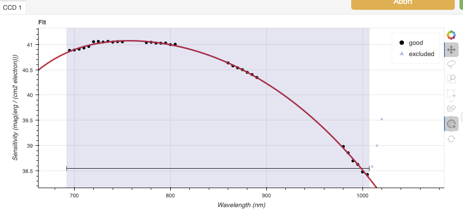
Again, here are the before and after fits. The x-axis this time is in wavelength with the blue-end to the left and the red-end to the right. The fits is good within the region that covers the first order. But there is some flaring at both ends with some on the red side due to our previous cut not being aggressive enough.

Like we did for the trace, we can define a region to use for the fit, this is the gray area on the “after” plot. Another thing that was adjusted is the order of the fit. The default is set to 6, and to avoid flaring on the blue-end, we can reduce the order to 4 to have the smooth function shown here.

7.2.11. Science Observations

The science target is a high redshift quasar. The sequence has three images that were dithered along the dispersion axis. DRAGONS will remove the sky from the three images using the nod-and-shuffle beams. The resulting 2D spectra will then be register and stacked before extraction.

This is what one raw image looks like.

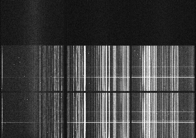
With the master bias, the master flat, the processed arcs (one for each of the grating position, aka central wavelength), and the processed standard in the local calibration manager, one only needs to do as follows to reduce the science observations and extract the 1-D spectrum.

reduce @sci.lis -p traceApertures:interactive=True

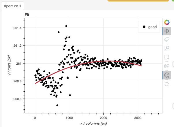
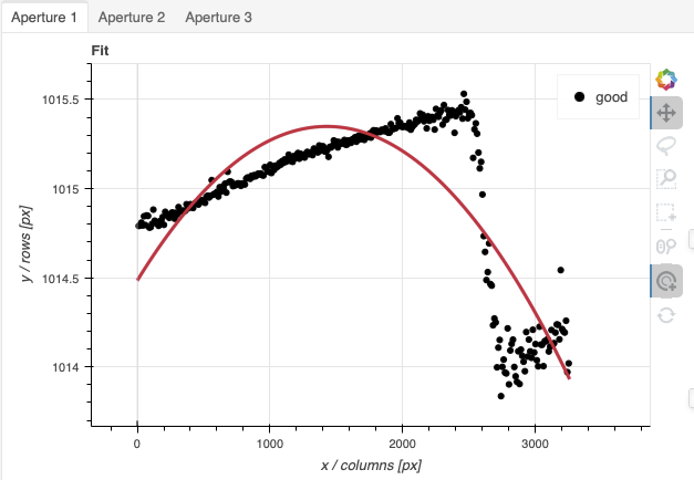
traceApertures

Below are the before and after adjustments plots. The x-axis is in pixel like before for the spectrophotometric standard but this time, the data has been resampled (for the stacking) before traceApertures is called. Because of that, blue is left and red is right.

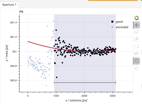
A sharp discontinuity is visible where the first order fades away and the second order starts showing up, around pixel 2600. We set the region to use only the first order light, the points left of the discontinuity.

This time however note that there are three apertures. You can see a tab for each one in the upper part of the plot. If you were not interested in the other, fainter sources, you could ignore them. But if the fainter sources were of interest, you would want to apply the same region to Aperture 2 and 3. The easiest way to do that is to set the region for Aperture 1, and then go to the “Regions” box at the bottom, copy the region, and then paste that region definition in the “Regions” box in the other two tabs.

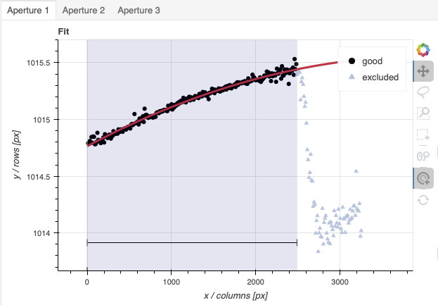
When done, click the green Accept button and the reduction will complete.

The product includes a 2-D spectrum (N20080830S0261_2D.fits) which has been bias corrected, flat fielded, QE-corrected, wavelength-calibrated, corrected for distortion, sky-subtracted, the beams combined, and then all frames stacked. It also produces the 1-D spectrum (N20080830S0261_1D.fits) extracted from that 2-D spectrum. The 1-D spectrum is flux calibrated with the sensitivity function from the spectrophotometric standard. The 1-D spectra are stored as 1-D FITS images in extensions of the output Multi-Extension FITS file.

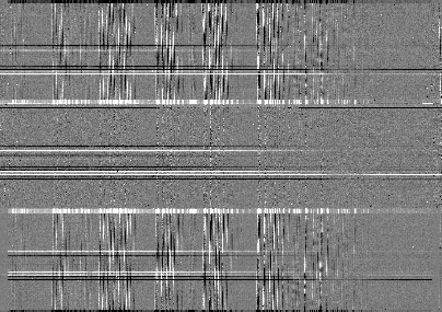
This is what the 2-D spectrum looks like. Only the middle section is valid.

reduce -r display N20080830S0261_2D.fits

Note

ds9 must be launched by the user ahead of running the display primitive. (ds9& on the terminal prompt.)

The apertures found are listed in the log for the findApertures primitive, just before the call to traceApertures. Information about the apertures are also available in the header of each extracted spectrum: XTRACTED, XTRACTLO, XTRACTHI, for aperture center, lower limit, and upper limit, respectively.

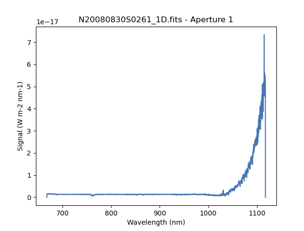
This is what the 1-D flux-calibrated spectrum of our sole target looks like.

dgsplot N20080830S0261_1D.fits 1

The entire spectrum is plotted including the part redder of the discontinuity where there is no light at all from the first order. What is there is whatever got caught in the extraction that followed the extrapolated trace.

The scaling of the plot is obviously wrong, but we can use the matplotlib interactive zooming feature to focus on the spectrum from the first order. That is shown in the plot on the right.

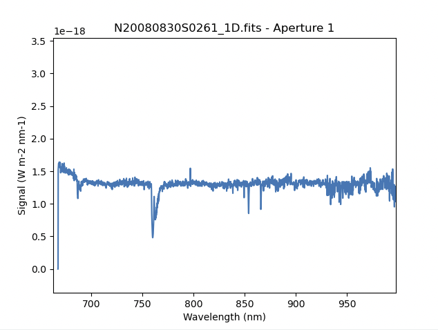
Note the flaring bluer of 700nm. This is because the spectrophotometric standard was observed with a central wavelength of 900nm and it is unable to constrain the sensitivity bluer of ~700nm. This can be seen in the plots of the interactive calculateSensitivity, the bluer point is at 690nm. (Processed Standard - Sensitivity Function) We have a science spectrum bluer of 690nm because of the other two central wavelength settings of 890nm and 880nm. Observing the standard with a central wavelength of 880nm would have help reduce, possible avoid entirely.