3.2. Example 1 - Star field with dithers - Using the “reduce” command line
In this example we will reduce a GMOS imaging observation of a star field using the “reduce” command that is operated directly from the unix shell. Just open a terminal and load the DRAGONS conda environment to get started.
The observations have been dithered.
3.2.1. The dataset
If you have not already, download and unpack the tutorial’s data package. Refer to Downloading the tutorial datasets for the links and simple instructions.
The dataset specific to this example is described in:
Here is a copy of the table for quick reference.
Science |
N20170614S0201-205
|
10 s, i-band
|
Bias |
N20170613S0180-184
N20170615S0534-538
|
|
Twilight Flats |
N20170702S0178-182
|
40 to 16 s, i-band
|
BPM |
bpm_20170306_gmos-n_Ham_22_full_12amp.fits
|
|
3.2.2. Set up the Calibration Service
Important
Remember to set up the calibration service.
Instructions to configure and use the calibration service are found in Setting up the Calibration Service, specifically the these sections: The Configuration File and Usage from the Command Line.
3.2.3. Check files
For this example, all the raw files we need are in the same directory called
../playdata/example1. Let us learn a bit about the data we have.
Ensure that you are in the playground directory and that the conda
environment that includes DRAGONS has been activated.
Let us call the command tool “typewalk”:
$ typewalk -d ../playdata/example1

directory:  /data/workspace/gmosimg_tutorial/playdata/example1
 N20170613S0180.fits ............... (AT_ZENITH) (AZEL_TARGET) (BIAS) (CAL) (GEMINI) (GMOS) (NON_SIDEREAL) (NORTH) (RAW) (UNPREPARED)
 ...
 N20170614S0201.fits ............... (GEMINI) (GMOS) (IMAGE) (NORTH) (RAW) (SIDEREAL) (UNPREPARED)
 ...
 N20170615S0534.fits ............... (AT_ZENITH) (AZEL_TARGET) (BIAS) (CAL) (GEMINI) (GMOS) (NON_SIDEREAL) (NORTH) (RAW) (UNPREPARED)
 ...
 N20170702S0182.fits ............... (CAL) (FLAT) (GEMINI) (GMOS) (IMAGE) (NORTH) (RAW) (SIDEREAL) (TWILIGHT) (UNPREPARED)
Done DataSpider.typewalk(..)
This command will open every FITS file within the folder passed after the -d
flag (recursively) and will print an unsorted table with the file names and the
associated tags. For example, calibration files will always have the CAL
tag. Flat images will always have the FLAT tag. This means that we can start
getting to know a bit more about our data set just by looking the tags. The
output above was trimmed for presentation.
3.2.4. Create File lists
This data set contains science and calibration frames. For some programs, it could have different observed targets and different exposure times depending on how you like to organize your raw data.
The DRAGONS data reduction pipeline does not organize the data for you. You have to do it. DRAGONS provides tools to help you with that.
The first step is to create lists that will be used in the data reduction process. For that, we use “dataselect”. Please, refer to the “dataselect” documentation for details regarding its usage.
First, navigate to the playground directory in the unpacked data package:
cd <path>/gmosim_tutorial/playground
3.2.4.1. List of Biases
The bias files are selected with “dataselect”:
$ dataselect --tags BIAS ../playdata/example1/*.fits -o list_of_bias.txt
3.2.4.2. List of Flats
Now we can do the same with the FLAT files:
$ dataselect --tags FLAT ../playdata/example1/*.fits -o list_of_flats.txt
If your dataset has flats obtained with more than one filter, you can add the
--expr 'filter_name=="i"' expression to get only the flats obtained within
the i-band. For example:
$ dataselect --tags FLAT --expr 'filter_name=="i"' ../playdata/example1/*.fits -o list_of_flats.txt
3.2.4.3. List for science data
The rest is the data with your science target. The simplest way, in this case, of creating a list of science frames is excluding everything that is a calibration:
$ dataselect --xtags CAL ../playdata/example1/*.fits -o list_of_science.txt
This will work for our dataset because we know that a single target was observed with a single filter and with the same exposure time. But what if we don’t know that?
We can check it by passing the “dataselect” output to the “showd” command
line using a “pipe” (|):
$ dataselect --expr 'observation_class=="science"' ../playdata/example1/*.fits | showd -d object,exposure_time
--------------------------------------------------------------------
filename                                      object   exposure_time
--------------------------------------------------------------------
../playdata/example1/N20170614S0201.fits   starfield            10.0
../playdata/example1/N20170614S0202.fits   starfield            10.0
../playdata/example1/N20170614S0203.fits   starfield            10.0
../playdata/example1/N20170614S0204.fits   starfield            10.0
../playdata/example1/N20170614S0205.fits   starfield            10.0
The -d flag tells “showd” which “descriptors” will be printed for
each input file. As you can see, we have only one target and only one
exposure time.
To select on target name and exposure time, specify the criteria in the
expr field of “dataselect”:
$ dataselect --expr '(object=="starfield" and exposure_time==10.)' ../playdata/example1/*.fits -o list_of_science.txt
We have our input lists and we have initialized the calibration database, we are ready to reduce the data.
Please make sure that you are still in the playground directory.
3.2.5. Bad Pixel Mask
Starting with DRAGONS v3.1, the bad pixel masks (BPMs) are now handled as calibrations. They are downloadable from the archive instead of being packaged with the software. They are automatically associated like any other calibrations. This means that the user now must download the BPMs along with the other calibrations and add the BPMs to the local calibration manager.
See Getting Bad Pixel Masks from the archive in Tips and Tricks to learn about the various ways to get the BPMs from the archive.
To add the static BPM included in the data package to the local calibration database:
caldb add ../playdata/example1/bpm*.fits
3.2.6. Create a Master Bias
We start the data reduction by creating a master bias for the science data. It can be created and added to the calibration database using the commands below:
$ reduce @list_of_bias.txt
The @ character before the name of the input file is the “at-file” syntax.
More details can be found in the "at-file" Facility documentation.
Because the database was given the “store” option in the dragonsrc file,
the processed bias will be automatically added to the database at the end of
the recipe.
To check that the master bias was added to the database, use caldb list.
Note
The file name of the output processed bias is the file name of the
first file in the list with _bias appended as a suffix. This the
general naming scheme used by “reduce”.
Note
If you wish to inspect the processed calibrations before adding them
to the calibration database, remove the “store” option attached to the
database in the dragonsrc configuration file. You will then have to
add the calibrations manually following your inspection, eg.
caldb add N20170613S0180_bias.fits
Note
The master bias will be saved in the same folder where reduce was
called and inside the ./calibrations/processed_bias folder. The latter
location is to cache a copy of the file. This applies to all the processed
calibration.
3.2.7. Create a Master Flat Field
Twilight flats images are used to produce an imaging master flat and the result is added to the calibration database.
$ reduce @list_of_flats.txt
Note “reduce” will query the local calibration manager for the master bias and use it in the data reduction.
3.2.8. Create Master Fringe Frame
Warning
The dataset used in this tutorial does not require fringe correction so we skip this step. To find out how to produce a master fringe frame, see Create Master Fringe Frame in the Tips and Tricks chapter.
3.2.9. Reduce Science Images
Once we have our calibration files processed and added to the database, we can
run reduce on our science data:
$ reduce @list_of_science.txt
This command will generate bias and flat corrected files and will stack them.
If a fringe frames is needed this command will apply the correction. The stacked
image will have the _image suffix.
The output stack units are in electrons (header keyword BUNIT=electrons). The output stack is stored in a multi-extension FITS (MEF) file. The science signal is in the “SCI” extension, the variance is in the “VAR” extension, and the data quality plane (mask) is in the “DQ” extension.
Below are one of the raw images and the final stack:
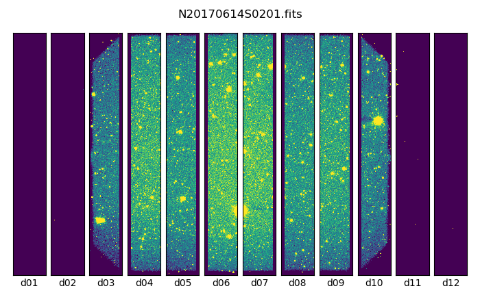
One of the multi-extensions files.
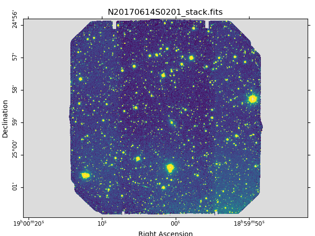
Final stacked image. The light-gray area represents the masked pixels.