5.3. Example 2 - J-band R3K Longslit Point Source - Using the “Reduce” class API

We will reduce a F2 R3K 1.25 m longslit observation the recurrent nova V1047 Cen using the Python programmatic interface.

This observation uses the 2-pixel slit. The dither pattern is a standard ABBA.

5.3.1. The dataset

If you have not already, download and unpack the tutorial’s data package. Refer to Downloading tutorial datasets for the links and simple instructions.

The dataset specific to this example is described in:

Example 2 - Datasets description

Here is a copy of the table for quick reference.

Science	S20190702S0107-110
Science darks (300s)	S20190706S0431-437
Science flat	S20190702S0111
Science flat darks (5s)	S20190629S0029-035
Science arc	S20190702S0112
Science arc darks (60s)	S20190629S0085-091
Science arc flat	Same as science flat
Telluric	S20190702S0099-102
Telluric darks (25s)	S20190706S0340-346
Telluric flat	Same as science flat
Telluric flat darks (16s)	Same as science flat darks
Telluric arc	S20190702S0103
Telluric arc darks	Same as science arc darks
Telluric arc flat	Same as telluric flat

5.3.2. Setting up

First navigate to your work directory in the unpacked data package.

cd <path>/f2ls_tutorial/playground

The first steps are to import libraries, set up the calibration manager, and set the logger.

5.3.2.1. Configuring the interactive interface

In ~/.dragons/, add the following to the configuration file dragonsrc:

[interactive]
browser = your_preferred_browser

The [interactive] section defines your preferred browser. DRAGONS will open the interactive tools using that browser. The allowed strings are “safari”, “chrome”, and “firefox”.

5.3.2.2. Importing libraries

import glob

import astrodata
import gemini_instruments
from recipe_system.reduction.coreReduce import Reduce
from gempy.adlibrary import dataselect

The dataselect module will be used to create file lists for the biases, the flats, the arcs, the telluric star, and the science observations. The Reduce class is used to set up and run the data reduction.

5.3.2.3. Setting up the logger

We recommend using the DRAGONS logger. (See also Double messaging issue.)

from gempy.utils import logutils
logutils.config(file_name='f2ls_tutorial.log')

5.3.2.4. Set up the Calibration Service

Important

Remember to set up the calibration service.

Instructions to configure and use the calibration service are found in Setting up the Calibration Service, specifically the these sections: The Configuration File and Usage from the API.

We recommend that you clean up your working directory (playground) and delete the old calibration database before you start. Create a fresh one.

Start a fresh calibration database (caldb.init(wipe=True)) when you start a new example.

5.3.3. Inspect and fix headers

It is unfortunately too common that the last frame of a science or telluric sequence gets some, not all, of its header values from the next (yes, future) frame which is normally, in the case of F2, a flat. The key headers to pay attention too are EXPTIME and LNRS. They are both associate with descriptors.

Let’s inspect the exposure_time and the read_mode for the science and the telluric data. For a given sequence, all the values should match.

First, we create is a list of all the files in the playdata directory.

all_files = glob.glob('../playdata/example2/*.fits')
all_files.sort()

We will select the telluric and science frames and display the values for the exposure_time and read_mode descriptors.

sciframes = dataselect.select_data(
    all_files,
    [],
    ['CAL'],
    dataselect.expr_parser('observation_class=="science"')
)
tellurics = dataselect.select_data(
    all_files,
    [],
    ['CAL'],
    dataselect.expr_parser('observation_class!="science"')
)

for f in sciframes:
    ad = astrodata.open(f)
    print(f"{f}:\t{ad.exposure_time()}\t{ad.read_mode()}")

for f in tellurics:
    ad = astrodata.open(f)
    print(f"{f}:\t{ad.exposure_time()}\t{ad.read_mode()}")

The science sequence:

../playdata/example2/S20190702S0107.fits           300.0           8
../playdata/example2/S20190702S0108.fits           300.0           8
../playdata/example2/S20190702S0109.fits           300.0           8
../playdata/example2/S20190702S0110.fits           300.0           8

The telluric sequence:

../playdata/example2/S20190702S0099.fits            25.0           1
../playdata/example2/S20190702S0100.fits            25.0           1
../playdata/example2/S20190702S0101.fits            25.0           1
../playdata/example2/S20190702S0102.fits            25.0           1

Everything looks good with all the exposure times and read modes matching. Had there been discrepancies, you would have fixed them as shown in Example 1 and Example 3.

5.3.4. Create file lists

This data set contains science and calibration frames. For some programs, it could contain different observed targets and different exposure times depending on how you like to organize your playdata/example2 data.

The DRAGONS data reduction pipeline does not organize the data for you. You have to do it. However, DRAGONS provides tools to help you.

The first step is to create input file lists. The tool “dataselect” helps with that. It uses Astrodata tags and “descriptors” to select the files and send the filenames to a text file that can then be fed to the Reduce class. (See the Astrodata User Manual for information about Astrodata and for a list of descriptors.)

Let’s get a fresh list of all the files in the playdata directory.

all_files = glob.glob('../playdata/example2/*.fits')
all_files.sort()

We will search that list for files with specific characteristics. We use the all_files list as an input to the function dataselect.select_data() . The function’s signature is:

select_data(inputs, tags=[], xtags=[], expression='True')

5.3.4.1. Several lists for the darks

The flats, the arcs, the telluric, and the science observations need a master dark matching their exposure time. We need a list of darks for each set. The exposure times are 5s for the flats, 60s for the arcs, 25s for the telluric frames, and 300s for the science frames.

A dark correction is unfortunately necessary for Flamingos 2 data due to strong and bright patterns that can interfere with the reduction if left present in the data.

exposure_times = [5, 25, 60, 300]
darks = {}
for exptime in exposure_times:
    darks[exptime] = dataselect.select_data(
            all_files,
            ['DARK'],
            [],
            dataselect.expr_parser(f'exposure_time=={exptime}')
    )

5.3.4.2. One list for the flat

Only one flat was obtained for this observation, one flat just after the science sequence. It can happen that a flat is also obtained after the telluric sequence. The recipe to make the master flats combines the input flats if more than one is passed. Therefore each flat group (one flat or flats taken in succession) needs to be reduced independently. Here, we just need to send the filename of the unique flat to a list.

Note

No selection criteria are needed here since there is just one flat. Obviously, if your raw data directory contains all the data for the entire program you will have to apply selection criteria to ensure that the flats are sorted adequately.

for f in dataselect.select_data(all_files, ['FLAT']):
    ad = astrodata.open(f)
    print(f"{f}\t{ad.ut_time()}\t{ad.disperser()}")

../playdata/example2/S20190702S0111.fits   01:54:39.300000

flat = dataselect.select_data(all_files, ['FLAT'])

5.3.4.3. A list for the arcs

There are two arcs. One for the telluric sequence, one for the science sequence. The recipe to measure the wavelength solution will not stack the arcs. Therefore, we can conveniently create just one list with all the raw arc observations in it and they will be processed independently.

arcs = dataselect.select_data(all_files, ['ARC'])

5.3.4.4. A list for the telluric

DRAGONS does not recognize the telluric star as such. This is because, at Gemini, the observations are taken like science data and the Flamingos 2 headers do not explicitly state that the observation is a telluric standard. In most cases, the observation_class descriptor can be used to differentiate the telluric from the science observations, along with the rejection of the CAL tag to reject flats and arcs.

tellurics = dataselect.select_data(
    all_files,
    [],
    ['CAL'],
    dataselect.expr_parser('observation_class!="science"')
)

5.3.4.5. A list for the science observations

The science observations can be selected from the observation class, science, that is how they are differentiated from the telluric standards which are partnerCal.

If we had multiple targets, we would need to split them into separate lists. To inspect what we have we can use dataselect.

all_science = dataselect.select_data(
    all_files,
    [],
    ['CAL'],
    dataselect.expr_parser('observation_class=="science"')
)
for sci in all_science:
    ad = astrodata.open(sci)
    print(sci, '  ', ad.object())

../playdata/example2/S20190702S0107.fits   V1047 Cen
../playdata/example2/S20190702S0108.fits   V1047 Cen
../playdata/example2/S20190702S0109.fits   V1047 Cen
../playdata/example2/S20190702S0110.fits   V1047 Cen

Here we only have one object from the same sequence. If we had multiple objects we could add the object name in the expression.

sciframes = dataselect.select_data(
    all_files,
    [],
    ['CAL'],
    dataselect.expr_parser('observation_class=="science" and object=="V1047 Cen"')
)

5.3.5. Master Darks

Now that the lists are created, we just need to run Reduce on each list.

for exptime in darks.keys():
    reduce_darks = Reduce()
    reduce_darks.files.extend(darks[exptime])
    reduce_darks.runr()

5.3.6. Master Flat Fields

Flamingos 2 longslit flat fields are normally obtained at night along with the observation sequence to match the telescope and instrument flexure.

Flamingos 2 longslit master flat fields are created from the lamp-on flat(s) and a master dark matching the flats exposure times. Lamp-off flats are not used.

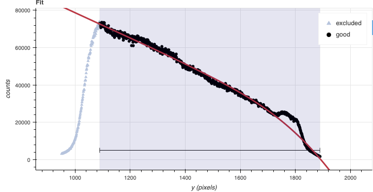
In Flamingos 2 spectroscopic observations a blocking filter is used. The sharp drops in signal at both end makes fitting a function difficult. Our recommendation is to set the region to be between the sharp drops and then fit a low-order cubic spline. This is a departure from what is being recommended for the other Gemini spectrographs where a high-order is recommended to fit all the wiggles.

For F2, only the overall shape should be fit. The detailed fitting will be taken care of when the sensitivity function is calculated using the telluric standard star.

We have defined appropriate defaults for the order and the region to use to normalize the flat for each grism and filter combinations. You should not have to modify them.

reduce_flats = Reduce()
reduce_flats.files.extend(flat)
reduce_flats.runr()

If you wish to see the fit, you can add reduce_flats.uparms = dict([('interactive', True)]) before the runr() call. For reference, this is how the flat fit looks like.

5.3.7. Processed Arc - Wavelength Solution

Obtaining the wavelength solution for Flamingos 2 is fairly straightforward from the user’s perspective. There are usually a sufficient number of lines in the lamp. Note, however, that the lines becomes asymmetric as they move away from the center. There are provisions in the algorithm to account of that effect but the precision of the solution is limited.

The recipe for the arc requires a flat as it contains a map of the unilluminated areas. The master dark is required because of the strong pattern that is often horizontal and that could be interpreted as an emission line if not removed.

The solution is normally found automatically, but it does not hurt to visually inspect it in interactive mode.

reduce_arcs = Reduce()
reduce_arcs.files.extend(arcs)
reduce_arcs.uparms = dict([('interactive', True),])
reduce_arcs.runr()

The interactive tools are introduced in section Interactive tools.

5.3.8. Telluric Standard

The telluric standard observed after the science observation is “hip 63036”. The spectral type of the star is A0/1V.

To properly calculate and fit a telluric model to the star, we need to know its effective temperature. To properly scale the sensitivity function (to use the star as a spectrophotometric standard), we need to know the star’s magnitude. Those are inputs to the fitTelluric primitive.

In Eric Mamajek’s list “A Modern Mean Dwarf Stellar Color and Effective Temperature Sequence” (https://www.pas.rochester.edu/~emamajek/EEM_dwarf_UBVIJHK_colors_Teff.txt) the effective temperature of an A0/1V star as about 9500 K. The precise value has only a small effect on the derived sensitivity and even less effect on the telluric correction, so the temperature from any reliable source can be used. Using Simbad, we find that the star has a magnitude of J=7.498, which is the closest waveband to our observation.

Note that the data are recognized by Astrodata as normal F2 longslit science spectra. To calculate the telluric correction, we need to specify the telluric recipe (reduceTelluric), otherwise the default science reduction will be run.

reduce_telluric = Reduce()
reduce_telluric.files.extend(tellurics)
reduce_telluric.recipename = 'reduceTelluric'
reduce_telluric.uparms = dict([
            ('fitTelluric:bbtemp', 9500),
            ('fitTelluric:magnitude', 'J=7.498'),
            ('fitTelluric:interactive', True),
            ('prepare:bad_wcs', 'new')
            ])
reduce_telluric.runr()

The prepare:bad_wcs=new is needed because the WCS in the raw data is not quite right and that leads to an incorrect sky subtraction and alignment. See Recognizing and fixing bad WCS for more information.

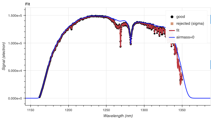
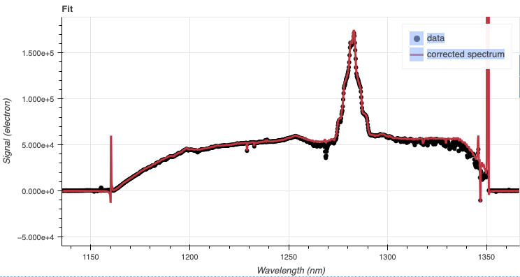
Using the defaults, the fit and model spectrum look like this:

5.3.9. Science Observations

The science target is recurrent nova. The observation is one ABBA set. DRAGONS will subtract the dark current, flatfield the data, apply the wavelength calibration, subtract the sky, stack the aligned spectra. Then the source will be extracted to a 1D spectrum, the telluric features removed, and the spectrum flux calibrated.

Following the wavelength calibration, the default recipe has an optional step to adjust the wavelength zero point using the sky lines. By default, this step will NOT make any adjustment. We found that in general, the adjustment is so small as being in the noise. If you wish to make an adjustment, or try it out, see Adjusting the Wavelength Zeropoint to learn how.

Note

When the algorithm detects multiple sources, all of them will be extracted. Each extracted spectrum is stored in an individual extension in the output multi-extension FITS file.

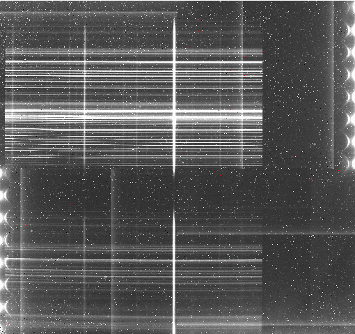
This is what one raw image looks like.

To run the reduction, call the Reduce class on the science list. The calibrations will be automatically associated. It is recommended to run the reduction in interactive mode to allow inspection of and control over the critical steps.

There are many sources along the slit. We know that we are interested only in the brightest one. Therefore, we set the maximum number of sources to find to 1 in findApertures.

reduce_science = Reduce()
reduce_science.files.extend(sciframes)
reduce_science.uparms = dict([
        ('interactive', True),
        ('prepare:bad_wcs', 'new'),
        ('findApertures:max_apertures', 1)
        ])
reduce_science.runr()

The exposure time of each of the four frames is 300 seconds. The default time interval for the sky subtraction association is 600 seconds. The default number of skies to use, min_skies is 2. The routine will issues warnings that it cannot find 2 sky frames compatible with the time interval. The default behavior in this case is to issue the warnings and ignore the time interval constraint. Here it works fine. Depending on the sky conditions and variability, another solution would be to set min_skies to 1 and always catch the A or B frame closest in time. Which works best for a given dataset is something the users will have to judge for themselves.

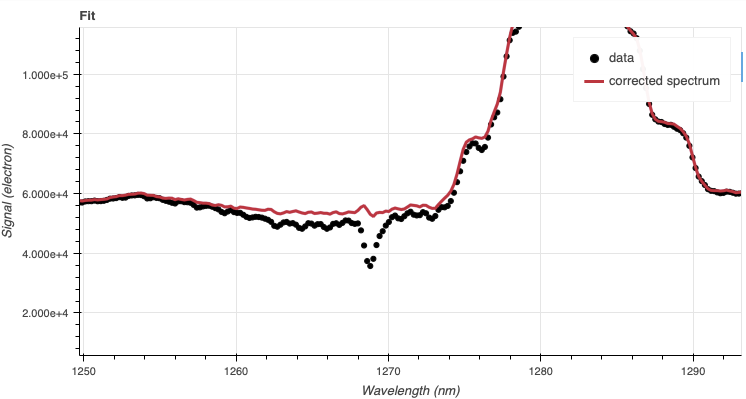
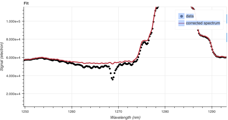
At the telluricCorrect step you should focus on the section illustrated below. The redder region is marked as non-illuminated in the flat and masked.

If you zoom-in on a region where there was a telluric feature, you will notice that the fit is not quite aligned. It happens, that is what the interactive tool for telluricCorrect is for. You can adjust the shift to get a better removal of the telluric feature.

A shift of -0.25 helps.

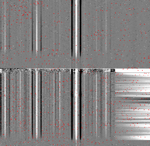
The 2D spectrum before extraction looks like this, with blue wavelengths at the bottom and the red-end at the top. Only the bottom half of the frame is valid and within the J filter transmission band.

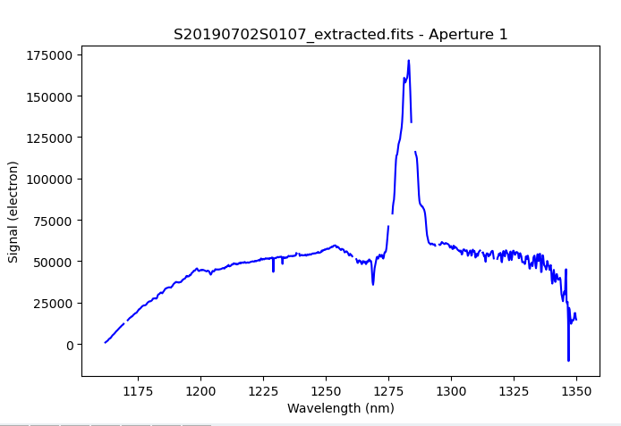
The 1D extracted spectrum before telluric correction or flux calibration, obtained by adding ('extractSpectra:write_outputs', True) to the uparms dictionary, looks like this.

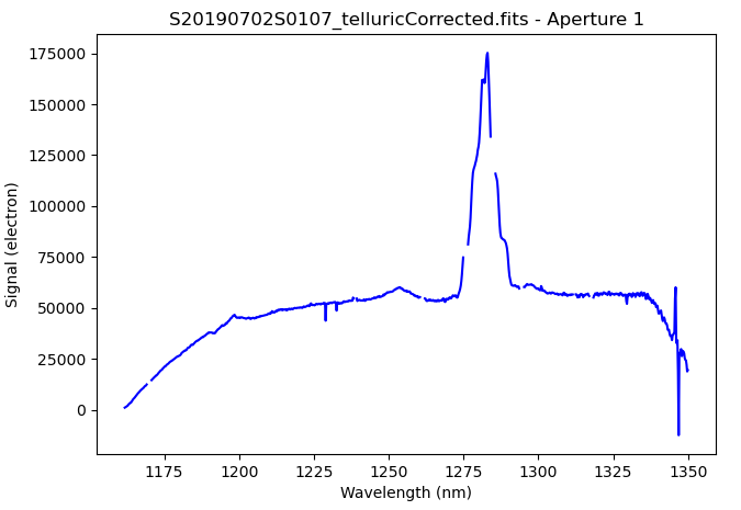
The 1D extracted spectrum after telluric correction but before flux calibration, obtained by adding ('telluricCorrect:write_outputs', True) to the uparms dictionary, looks like this.

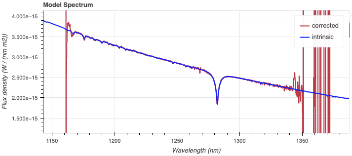
And the final spectrum, corrected for telluric features and flux calibrated.

from gempy.adlibrary import plotting
ad = astrodata.open(reduce_science.output_filenames[0])
plotting.dgsplot_matplotlib(ad, 1, kwargs={})

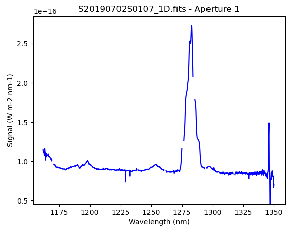
The “notch” in the emission line is where pixels have been masked, in this case due to saturation (probably when a bright sky line added to the star’s signal to push the counts over the limit). The tool dgsplot understands the data quality plane and plots the spectrum accordingly.