4.3. Example 1 - JH and HK Longslit Point Source - Using the “Reduce” class API

We will reduce a Flamingos 2 JH and a HK longslit observation of the 2022 eruption of the recurrent nova U Sco using the Python programmatic interface.

The 2-pixel slit is used. The dither sequence is ABBA-ABBA.

4.3.1. The dataset

If you have not already, download and unpack the tutorial’s data package. Refer to Downloading tutorial datasets for the links and simple instructions.

The dataset specific to this example is described in:

Example 1 - Datasets description

4.3.2. Setting up

First navigate to your work directory in the unpacked data package.

cd <path>/f2ls_tutorial/playground

The first steps are to import libraries, set up the calibration manager, and set the logger.

4.3.2.1. Configuring the interactive interface

In ~/.dragons/, add the following to the configuration file dragonsrc:

[interactive]
browser = your_preferred_browser

The [interactive] section defines your preferred browser. DRAGONS will open the interactive tools using that browser. The allowed strings are “safari”, “chrome”, and “firefox”.

4.3.2.2. Importing libraries

import glob

import astrodata
import gemini_instruments
from recipe_system.reduction.coreReduce import Reduce
from gempy.adlibrary import dataselect

The dataselect module will be used to create file lists for the biases, the flats, the arcs, the telluric star, and the science observations. The Reduce class is used to set up and run the data reduction.

4.3.2.3. Setting up the logger

We recommend using the DRAGONS logger. (See also Double messaging issue.)

from gempy.utils import logutils
logutils.config(file_name='f2ls_tutorial.log')

4.3.2.4. Set up the Calibration Service

Important

Remember to set up the calibration service.

Instructions to configure and use the calibration service are found in Setting up the Calibration Service, specifically the these sections: The Configuration File and Usage from the API.

We recommend that you clean up your working directory (playground) and delete the old calibration database before you start. Create a fresh one.

Start a fresh calibration database (caldb.init(wipe=True)) when you start a new example.

4.3.3. Inspect and fix headers

It is unfortunately too common that the last frame of a science or telluric sequence gets some, not all, of its header values from the next (yes, future) frame which is normally, in the case of F2, a flat. The key headers to pay attention too are EXPTIME and LNRS. They are both associate with descriptors.

Let’s inspect the exposure_time and the read_mode for the science and the telluric data. For a given sequence, all the values should match.

First, we create is a list of all the files in the playdata directory.

all_files = glob.glob('../playdata/example1/*.fits')
all_files.sort()

We will select the telluric and science frames and display the values for the exposure_time and read_mode descriptors.

telJH = dataselect.select_data(
    all_files,
    [],
    ['CAL'],
    dataselect.expr_parser('observation_class=="partnerCal" and disperser=="JH"')
)
telHK = dataselect.select_data(
    all_files,
    [],
    ['CAL'],
    dataselect.expr_parser('observation_class=="partnerCal" and disperser=="HK"')
)
sciJH = dataselect.select_data(
    all_files,
    [],
    ['CAL'],
    dataselect.expr_parser('observation_class=="science" and disperser=="JH"')
)
sciJH = dataselect.select_data(
    all_files,
    [],
    ['CAL'],
    dataselect.expr_parser('observation_class=="science" and disperser=="HK"')
)

for f in telJH:
    ad = astrodata.open(f)
    print(f"{f}:\t{ad.exposure_time()}\t{ad.read_mode()}")

for f in telHK:
    ad = astrodata.open(f)
    print(f"{f}:\t{ad.exposure_time()}\t{ad.read_mode()}")

for f in sciJH:
    ad = astrodata.open(f)
    print(f"{f}:\t{ad.exposure_time()}\t{ad.read_mode()}")

for f in sciJH:
    ad = astrodata.open(f)
    print(f"{f}:\t{ad.exposure_time()}\t{ad.read_mode()}")

You will notice that the exposure times and read mode for each sequence match, except for the HK science sequence where the last frame claims to have an exposure time of 90 seconds instead of 25, and a read mode of 1 (LNRS keyword) instead of 4. Those are the values that apply to the next frame, the flat. The data was taken with the correct exposure time and read mode, but the headers are wrong.

../playdata/example1/S20220617S0038.fits            25.0           4
../playdata/example1/S20220617S0039.fits            25.0           4
../playdata/example1/S20220617S0040.fits            25.0           4
../playdata/example1/S20220617S0041.fits            90.0           1

Let’s fix that. So that you can rerun these same commands before, we first make a copy of the problematic file and give it a new name, leaving the original untouched. Obviously, with your own data, you would just fix the downloaded file once and for all, skipping the copy.

import shutil
shutil.copy('../playdata/example1/S20220617S0041.fits', '../playdata/example1/S20220617S0041_fixed.fits')

ad = astrodata.open('../playdata/example1/S20220617S0041_fixed.fits')
ad.phu['EXPTIME'] = 25
ad.phu['LNRS'] = 4
ad.write(overwrite=True)

4.3.4. Create file lists

This data set contains science and calibration frames. For some programs, it could contain different observed targets and different exposure times depending on how you like to organize your raw data.

The DRAGONS data reduction pipeline does not organize the data for you. You have to do it. However, DRAGONS provides tools to help you.

The first step is to create input file lists. The module “dataselect” helps. It uses Astrodata tags and “descriptors” to select the files and send the filenames to a text file that can then be fed to the Reduce class. (See the Astrodata User Manual for information about Astrodata and for a list of descriptors.)

Let’s get a fresh list of all the files in the playdata directory.

all_files = glob.glob('../playdata/example1/*.fits')
all_files.sort()

We will search that list for files with specific characteristics. We use the all_files list as an input to the function dataselect.select_data() . The function’s signature is:

select_data(inputs, tags=[], xtags=[], expression='True')

4.3.4.1. Several lists for the darks

The flats, the arcs, the telluric, and the science observations need a master dark matching their exposure time. We need a list of darks for each set, and for both JH and HK gratings.

A dark correction is unfortunately necessary for Flamingos 2 data due to strong and bright patterns that can interfere with the reduction if left present in the data.

exposure_times = [6, 8, 15, 18, 25, 60, 90]
darks = {}
for exptime in exposure_times:
    darks[exptime] = dataselect.select_data(
            all_files,
            ['DARK'],
            [],
            dataselect.expr_parser(f'exposure_time=={exptime}')
    )

4.3.4.2. Four lists for the flats

We have four observation sequences: science and telluric for both JH and HK settings. Each has its own flat. The recipe to make the master flats will combine the flats more than one is passed. We need each flat to be processed independently as they were taken at a slightly different telescope orientation. Therefore we need to separate them into four lists.

There are various ways to do that with dataselect. Here use the name of the disperser and a UT time selection.

We first check the times at which the flats were taken. Then use that information to set our selection criteria to separate them.

for f in dataselect.select_data(all_files, ['FLAT']):
    ad = astrodata.open(f)
    print(f"{f}\t{ad.ut_time()}\t{ad.disperser()}")

../playdata/example1/S20220617S0031.fits    00:30:30.100000 HK_G5802
../playdata/example1/S20220617S0042.fits    00:57:17.100000 HK_G5802
../playdata/example1/S20220617S0048.fits    01:06:37.100000 JH_G5801
../playdata/example1/S20220617S0077.fits    01:58:44.100000 JH_G5801

For HK, the telluric was taken before the science, for JH, it was taken after. Therefore, we can construct our lists this way:

flatsciJH = dataselect.select_data(
    all_files,
    ['FLAT'],
    [],
    dataselect.expr_parser('filter_name=="JH" and ut_time<="01:56:00"')
)
flattelJH = dataselect.select_data(
    all_files,
    ['FLAT'],
    [],
    dataselect.expr_parser('filter_name=="JH" and ut_time>="01:56:00"')
)
flatsciHK = dataselect.select_data(
    all_files,
    ['FLAT'],
    [],
    dataselect.expr_parser('filter_name=="HK" and ut_time>="00:52:00"')
)
flattelHK = dataselect.select_data(
    all_files,
    ['FLAT'],
    [],
    dataselect.expr_parser('filter_name=="HK" and ut_time<="00:52:00"')
)

The exact UT time does not matter as long as it is between the two flats that we want to separate.

4.3.4.3. A list for the arcs

There are four arcs. One for the telluric sequence, one for the science sequence, and for both the JH and HK gratings. The recipe to measure the wavelength solution will not stack the arcs. Therefore, we can conveniently create just one list with all the raw arc observations in it and they will be processed independently.

arcs = dataselect.select_data(all_files, ['ARC'])

4.3.4.4. A list for the telluric

DRAGONS does not recognize the telluric star as such. This is because, at Gemini, the observations are taken like science data and the Flamingos 2 headers do not explicitly state that the observation is a telluric standard. In most cases, the observation_class descriptor can be used to differentiate the telluric from the science observations, along with the rejection of the CAL tag to reject flats and arcs.

telluricsJH = dataselect.select_data(
    all_files,
    [],
    ['CAL'],
    dataselect.expr_parser('observation_class=="partnerCal" and disperser=="JH"')
)
telluricsHK = dataselect.select_data(
    all_files,
    [],
    ['CAL'],
    dataselect.expr_parser('observation_class=="partnerCal" and disperser=="HK"')
)

4.3.4.5. A list for the science observations

The science observations can be selected from the observation class, science, that is how they are differentiated from the telluric standards which are partnerCal.

If we had multiple targets, we would need to split them into separate lists. To inspect what we have we can use dataselect.

all_science = dataselect.select_data(
    all_files,
    [],
    ['CAL'],
    dataselect.expr_parser('observation_class=="science"')
)
for sci in all_science:
    ad = astrodata.open(sci)
    print(sci, '  ', ad.object())

../playdata/example1/S20220617S0038.fits    V* U Sco
../playdata/example1/S20220617S0039.fits    V* U Sco
../playdata/example1/S20220617S0040.fits    V* U Sco
../playdata/example1/S20220617S0041.fits    V* U Sco
../playdata/example1/S20220617S0041_fixed.fits    V* U Sco
../playdata/example1/S20220617S0044.fits    V* U Sco
../playdata/example1/S20220617S0045.fits    V* U Sco
../playdata/example1/S20220617S0046.fits    V* U Sco
../playdata/example1/S20220617S0047.fits    V* U Sco

Also, since we had to fix the exposure time for one of the files and we created a copy instead of changing the original, we need to make sure only the science frame with the correct exposure time of 25 seconds get picked up. If you had fixed the original, mostly likely what you will do with your own data, you wouldn’t need to select on the exposure time.

sciJH = dataselect.select_data(
    all_files,
    [],
    ['CAL'],
    dataselect.expr_parser('observation_class=="science" and disperser=="JH" and object=="V* U Sco"')
)
sciHK = dataselect.select_data(
    all_files,
    [],
    ['CAL'],
    dataselect.expr_parser('observation_class=="science" and disperser=="HK" and exposure_time==25 and object=="V* U Sco"')
)

4.3.5. Master Darks

Now that the lists are created, we just need to run Reduce on each list.

for exptime in darks.keys():
    reduce_darks = Reduce()
    reduce_darks.files.extend(darks[exptime])
    reduce_darks.runr()

4.3.6. Master Flat Fields

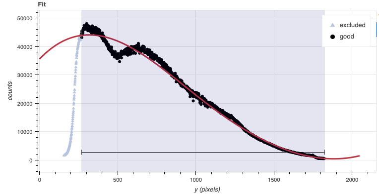
Flamingos 2 longslit flat fields are normally obtained at night along with the observation sequence to match the telescope and instrument flexure.

Flamingos 2 longslit master flat fields are created from the lamp-on flat(s) and a master dark matching the flats exposure times. Lamp-off flats are not used.

In Flamingos 2 spectroscopic observations a blocking filter is used. The sharp drops in signal at both end makes fitting a function difficult. Our recommendation is to set the region to be between the sharp drops and then fit a low-order cubic spline. This is a departure from what is being recommended for the other Gemini spectrograph where a high-order is recommended to fit all the wiggles.

For F2, only the overall shape should be fit. The detailed fitting will be taken care of when the sensitivity function is calculated using the telluric standard star.

We have defined appropriate defaults for the order and the region to use to normalize the flat for each grism and filter combinations. You should not have to modify them.

flatlists = [flatsciJH, flattelJH, flatsciHK, flattelHK]
for flats in flatlists:
    reduce_flats = Reduce()
    reduce_flats.files.extend(flats)
    reduce_flats.runr()

If you wish to see the fit, you can add reduce_flats.uparms = dict([('interactive', True)]) before the runr() call. For reference, this is how the HK flat fit looks like.

4.3.7. Processed Arc - Wavelength Solution

Obtaining the wavelength solution for Flamingos 2 is fairly straightforward from the user’s perspective. There are usually a sufficient number of lines in the lamp. Note, however, that the lines becomes asymmetric as they move away from the center. There are provisions in the algorithm to account of that effect but the precision of the solution is limited.

The recipe for the arc requires a flat as it contains a map of the unilluminated areas. The master dark is required because of the strong pattern that is often horizontal and that could be interpreted as an emission line if not removed.

The solution is normally found automatically, but it does not hurt to visually inspect it in interactive mode.

reduce_arcs = Reduce()
reduce_arcs.files.extend(arcs)
reduce_arcs.uparms = dict([('interactive', True),])
reduce_arcs.runr()

The interactive tools are introduced in section Interactive tools.

4.3.8. Telluric Standards

Two telluric standards are required for the reduction of this data set. The HK observations were done at the beginning of the program’s sequence. A HK telluric was observed before the start of the science sequence. The JH observations were done at the end of the sequence and the matching JH telluric was obtained afterwards.

The JH telluric is HIP 83920, a A0V star with an estimated temperature of 9700K and a H magnitude of 8.044. The HK telluric is HIP 79156, a A0.5V star with an estimated temperature of 9500K and a H magnitude of 7.576.

(Temperatures from Eric Mamajek’s list “A Modern Mean Dwarf Stellar Color and Effective Temperature Sequence” https://www.pas.rochester.edu/~emamajek/EEM_dwarf_UBVIJHK_colors_Teff.txt )

Those physical characteristic are required to properly calculate and fit a telluric model to the star and scale the sensitivity function. They are fed to the primitive fitTelluric.

Note that the data are recognized by Astrodata as normal F2 longslit science spectra. To calculate the telluric correction, we need to specify the telluric recipe (reduceTelluric), otherwise the default science reduction will be run.

reduce_telluricJH = Reduce()
reduce_telluricJH.files.extend(telluricsJH)
reduce_telluricJH.recipename = 'reduceTelluric'
reduce_telluricJH.uparms = dict([
            ('fitTelluric:bbtemp', 9700),
            ('fitTelluric:magnitude', 'H=8.044'),
            ('fitTelluric:interactive', True),
            ])
reduce_telluricJH.runr()

reduce_telluricHK = Reduce()
reduce_telluricHK.files.extend(telluricsHK)
reduce_telluricHK.recipename = 'reduceTelluric'
reduce_telluricHK.uparms = dict([
            ('fitTelluric:bbtemp', 9500),
            ('fitTelluric:magnitude', 'H=8.576'),
            ('fitTelluric:interactive', True),
            ('prepare:bad_wcs', 'new')
            ])
reduce_telluricHK.runr()

The WCS for the HK data are incorrect, hence the prepare:bad_wcs=new option. See Recognizing and fixing bad WCS for more information.

The JH fit looks like this:

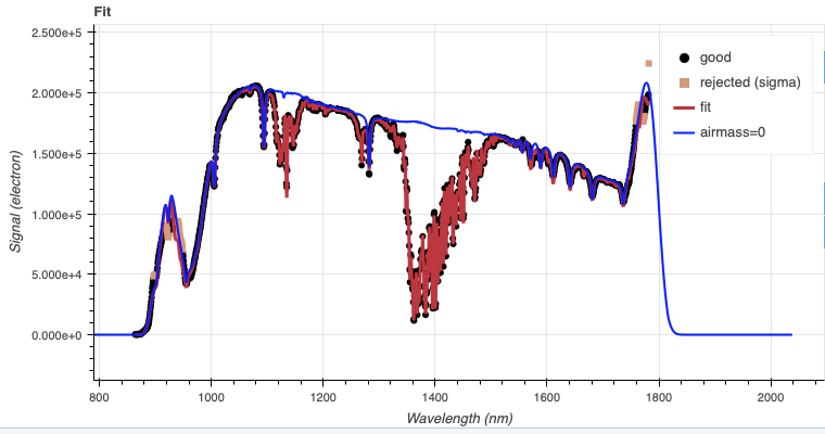
The flare up on the red end is the second order peeking through. The sharp dip in the blue is due to a large and bright artifact (likely a reflection) that is seen in all the JH frames and can be clearly seen in the normalized flat field that we produced earlier. The position of the artifact is stable but its strength does not seem to be as it is never completely removed during flat fielding.

Similar observations can be made about the HK data. In the HK data, the reflection artifact is softer but present nonetheless. Screenshots are available here: Reflections in flats

4.3.9. Science Observations

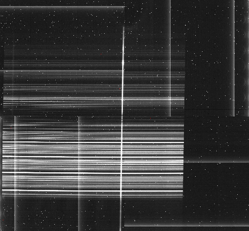
The target is a recurrent nova, U Sco, that was going through an eruption at the time of the observations. The dither pattern is a standard ABBA, repeated once.

DRAGONS will subtract the dark current, flatfield the data, apply the wavelength calibration, subtract the sky, stack the aligned spectra. Then the source will be extracted to a 1D spectrum, the telluric features removed, and the spectrum flux calibrated.

Following the wavelength calibration, the default recipe has an optional step to adjust the wavelength zero point using the sky lines. By default, this step will NOT make any adjustment. We found that in general, the adjustment is so small as being in the noise. If you wish to make an adjustment, or try it out, see Adjusting the Wavelength Zeropoint to learn how.

Note

When the algorithm detects multiple sources, all of them will be extracted. Each extracted spectrum is stored in an individual extension in the output multi-extension FITS file.

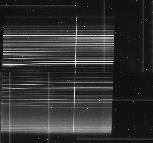
This is what the raw images looks like, for JH and for HK.

To run the reduction, call the Reduce class on the science list. The calibrations will be automatically associated. It is recommended to run the reduction in interactive mode to allow inspection of and control over the critical steps.

reduce_scienceJH = Reduce()
reduce_scienceJH.files.extend(sciJH)
reduce_scienceJH.uparms = dict([
        ('interactive', True),
        ('prepare:bad_wcs', 'new'),
        ])
reduce_scienceJH.runr()

reduce_scienceHK = Reduce()
reduce_scienceHK.files.extend(sciHK)
reduce_scienceHK.uparms = dict([
        ('interactive', True),
        ('prepare:bad_wcs', 'new'),
        ])
reduce_scienceHK.runr()

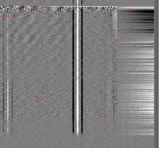
The 2D spectrum before extraction looks like this, with blue wavelengths at the bottom and the red-end at the top.

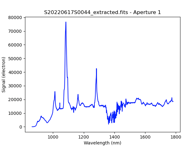
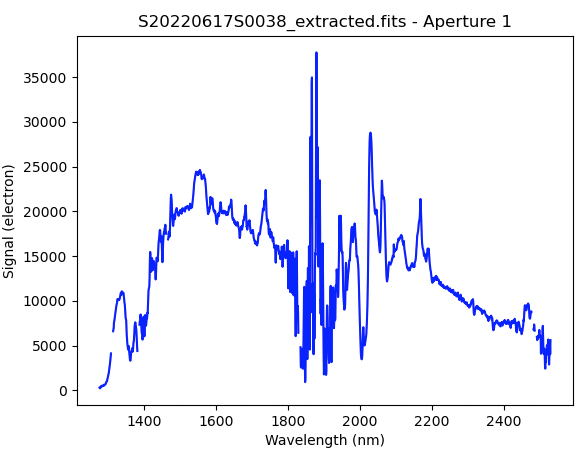
The 1D extracted spectra before telluric correction or flux calibration, obtained by adding ('extractSpectra:write_outputs', True) to the uparms dictionary, look like this.

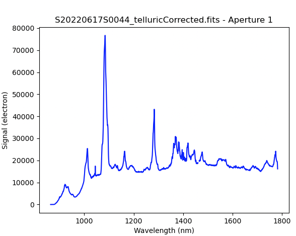
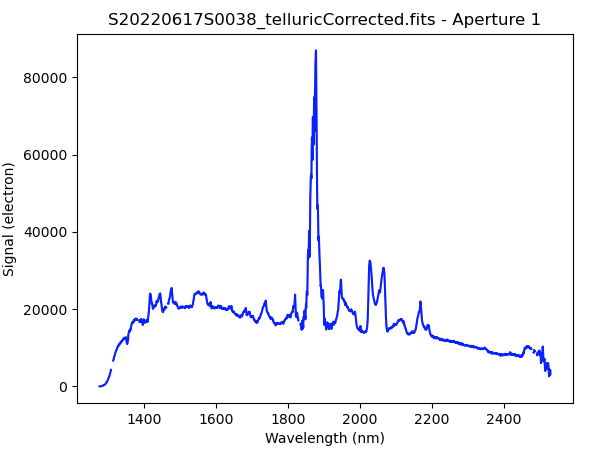
The 1D extracted spectra after telluric correction but before flux calibration, obtained by adding ('telluricCorrect:write_outputs', True) to the uparms dictionary, look like this.

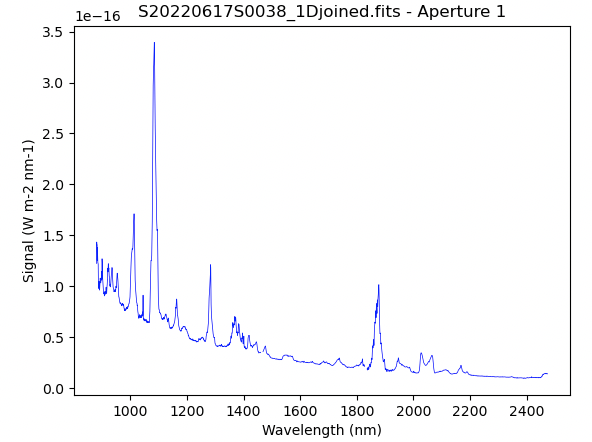
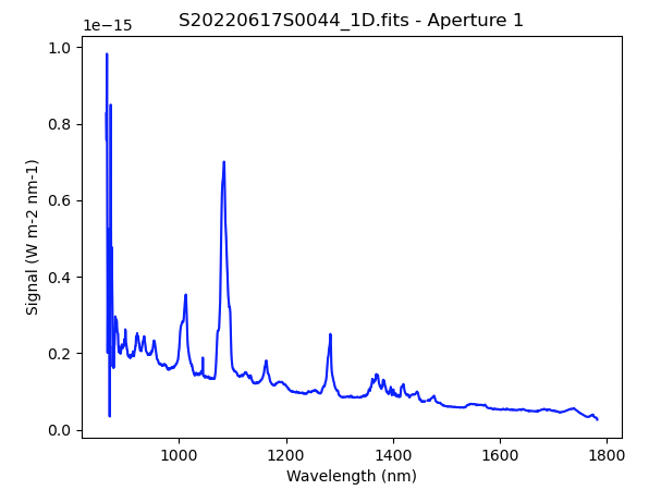
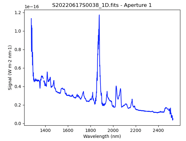
And the final spectra, corrected for telluric features and flux calibrated.

from gempy.adlibrary import plotting
ad = astrodata.open(reduce_scienceJH.output_filenames[0])
plotting.dgsplot_matplotlib(ad, 1, kwargs={})

ad = astrodata.open(reduce_scienceHK.output_filenames[0])
plotting.dgsplot_matplotlib(ad, 1, kwargs={})

To join the JH and HK spectra into a full range spectrum, we will use the joinSpectra recipe.

However, because of the low signal at the red and blue edges, it is not unusual for the flux calibration to diverge at the extremities; the function is simply not well constrained there. Therefore, before we join the spectra, it is recommended to mask the noisy extremities, and in this case the JH second order that was discussed above during the telluric reduction. We can use the dgsplot as above to identify the wavelength range we want to keep. Then we call maskBeyondRegions:

reduce_maskedges = Reduce()
reduce_maskedges.files.append('S20220617S0044_1D.fits')
reduce_maskedges.recipename = "maskBeyondRegions"
reduce_maskedges.uparms = dict([('regions', "880:1720")])
reduce_maskedges.runr()

reduce_maskedges = Reduce()
reduce_maskedges.files.append('S20220617S0038_1D.fits')
reduce_maskedges.recipename = "maskBeyondRegions"
reduce_maskedges.uparms = dict([('regions', "1400:2475")])
reduce_maskedges.runr()

We can now join the two cleaned up spectra.

reduce_join = Reduce()
reduce_join.files.extend(['S20220617S0044_regionsMasked.fits', 'S20220617S0038_regionsMasked.fits'])
reduce_join.recipename = "joinSpectra"
reduce_join.runr()

from gempy.adlibrary import plotting
ad = astrodata.open(reduce_join.output_filenames[0])
plotting.dgsplot_matplotlib(ad, 1, kwargs={})