4.3. Example 1 - Extended source with offset to sky - Using the “Reduce” class

A reduction can be initiated from the command line as shown in Example 1 - Extended source with offset to sky - Using the “reduce” command line and it can also be done programmatically as we will show here. The classes and modules of the RecipeSystem can be accessed directly for those who want to write Python programs to drive their reduction. In this example we replicate the command line version of Example 1 but using the Python programmatic interface. What is shown here could be packaged in modules for greater automation.

4.3.1. The dataset

If you have not already, download and unpack the tutorial’s data package. Refer to Downloading the tutorial datasets for the links and simple instructions.

The dataset specific to this example is described in:

Example 1 - Datasets descriptions.

Here is a copy of the table for quick reference.

Science	N20160102S0270-274 (on-target) N20160102S0275-279 (on-sky)
Science darks	N20160102S0423-432 (20 sec, like Science)
Flats	N20160102S0373-382 (lamps-on) N20160102S0363-372 (lamps-off)
Short darks	N20160103S0463-472
Standard star	N20160102S0295-299
BPM	bpm_20010317_niri_niri_11_full_1amp.fits

4.3.2. Setting up

First, navigate to your work directory in the unpacked data package.

cd <path>/nirils_tutorial/playground

The first steps are to import libraries, set up the calibration manager, and set the logger.

4.3.2.1. Importing libraries

import glob

import astrodata
import gemini_instruments
from recipe_system.reduction.coreReduce import Reduce
from gempy.adlibrary import dataselect

The dataselect module will be used to create file lists for the darks, the flats and the science observations. The Reduce class is used to set up and run the data reduction.

4.3.2.2. Setting up the logger

We recommend using the DRAGONS logger. (See also Double messaging issue.)

from gempy.utils import logutils
logutils.config(file_name='niriim_tutorial.log')

4.3.2.3. Set up the Calibration Service

Important

Remember to set up the calibration service.

Instructions to configure and use the calibration service are found in Setting up the Calibration Service, specifically the these sections: The Configuration File and Usage from the API.

4.3.3. Create file lists

The next step is to create input file lists. The module dataselect helps with that. It uses Astrodata tags and descriptors to select the files and store the filenames to a Python list that can then be fed to the Reduce class. (See the Astrodata User Manual for information about Astrodata and for a list of descriptors.)

The first list we create is a list of all the files in the playdata/example1 directory.

all_files = glob.glob('../playdata/example1/*.fits')
all_files.sort()

We will search that list for files with specific characteristics. We use the all_files list as an input to the function dataselect.select_data() . The function’s signature is:

select_data(inputs, tags=[], xtags=[], expression='True')

We show several usage examples below.

4.3.3.1. Two lists for the darks

We have two sets of darks; one set for the science frames, the 20-second darks, and another for making the BPM, the 1-second darks. We will create two lists.

If you did not know the exposure times for the darks, you could use dataselect as follows to see the exposure times of all the darks in the directory. We use the tag DARK and the descriptor exposure_time.

all_darks = dataselect.select_data(all_files, ['DARK'])
for dark in all_darks:
    ad = astrodata.open(dark)
    print(dark, '  ', ad.exposure_time())

../playdata/example1/N20160102S0423.fits    20.002
../playdata/example1/N20160102S0424.fits    20.002
../playdata/example1/N20160102S0425.fits    20.002
../playdata/example1/N20160102S0426.fits    20.002
../playdata/example1/N20160102S0427.fits    20.002
../playdata/example1/N20160102S0428.fits    20.002
../playdata/example1/N20160102S0429.fits    20.002
../playdata/example1/N20160102S0430.fits    20.002
../playdata/example1/N20160102S0431.fits    20.002
../playdata/example1/N20160102S0432.fits    20.002
../playdata/example1/N20160103S0463.fits    1.001
../playdata/example1/N20160103S0464.fits    1.001
../playdata/example1/N20160103S0465.fits    1.001
../playdata/example1/N20160103S0466.fits    1.001
../playdata/example1/N20160103S0467.fits    1.001
../playdata/example1/N20160103S0468.fits    1.001
../playdata/example1/N20160103S0469.fits    1.001
../playdata/example1/N20160103S0470.fits    1.001
../playdata/example1/N20160103S0471.fits    1.001
../playdata/example1/N20160103S0472.fits    1.001

As one can see above the exposure times all have a small fractional increment. This is just a floating point inaccuracy somewhere in the software that generates the raw NIRI FITS files. As far as we are concerned here in this tutorial, we are dealing with 20-second and 1-second darks. The function dataselect is smart enough to match those exposure times as “close enough”. So, in our selection expression, we can use “1” and “20” and ignore the extra digits.

Note

If a perfect match to 1.001 were required, simply set the argument strict to True in dataselect.expr_parser, eg. dataselect.expr_parser(expression, strict=True).

Let us create our two lists now. The filenames will be stored in the variables darks1s and darks20s.

darks1s = dataselect.select_data(
    all_files,
    ['DARK'],
    [],
    dataselect.expr_parser('exposure_time==1')
)

darks20s = dataselect.select_data(
    all_files,
    ['DARK'],
    [],
    dataselect.expr_parser('exposure_time==20')
)

Note

All expression need to be processed with dataselect.expr_parser.

4.3.3.2. A list for the flats

The flats are a sequence of lamp-on and lamp-off exposures. We just send all of them to one list.

flats = dataselect.select_data(all_files, ['FLAT'])

4.3.3.3. A list for the standard star

The standard star sequence is a series of datasets identified as “FS 17”. There are no keywords in the NIRI header identifying this target as a special standard star target. We need to use the target name to select only observations from that star and not our science target.

stdstar = dataselect.select_data(
    all_files,
    [],
    [],
    dataselect.expr_parser('object=="FS 17"')
)

4.3.3.4. A list for the science observations

The science frames are all IMAGE non-FLAT that are also not the standard. Since flats are tagged FLAT and IMAGE, we need to exclude the FLAT tag.

This translate to the following sequence:

target = dataselect.select_data(
    all_files,
    ['IMAGE'],
    ['FLAT'],
    dataselect.expr_parser('object!="FS 17"')
)

One could have used the name of the science target too, like we did for selecting the standard star observation in the previous section. The example above shows how to exclude a tag if needed and was considered more educational.

4.3.4. Master Dark

We first create the master dark for the science target, then add it to the calibration database. The name of the output master dark is N20160102S0423_dark.fits. The output is written to disk and its name is stored in the Reduce instance. The calibration service expects the name of a file on disk.

reduce_darks = Reduce()
reduce_darks.files.extend(darks20s)
reduce_darks.runr()

The Reduce class is our reduction “controller”. This is where we collect all the information necessary for the reduction. In this case, the only information necessary is the list of input files which we add to the files attribute. The Reduce.runr() method is where the recipe search is triggered and where it is executed.

Note

The file name of the output processed dark is the file name of the first file in the list with _dark appended as a suffix. This is the general naming scheme used by the Recipe System.

Note

If you wish to inspect the processed calibrations before adding them

to the calibration database, remove the “store” option attached to the database in the dragonsrc configuration file. You will then have to add the calibrations manually following your inspection, eg.

caldb.add_cal(reduce_darks.output_filenames[0])

4.3.5. Bad Pixel Mask

Starting with DRAGONS v3.1, the static bad pixel masks (BPMs) are now handled as calibrations. They are downloadable from the archive instead of being packaged with the software. They are automatically associated like any other calibrations. This means that the user now must download the BPMs along with the other calibrations and add the BPMs to the local calibration manager.

See Getting Bad Pixel Masks from the archive in Tips and Tricks to learn about the various ways to get the BPMs from the archive.

To add the BPM included in the data package to the local calibration database:

for bpm in dataselect.select_data(all_files, ['BPM']):
    caldb.add_cal(bpm)

The user can also create a supplemental, fresher BPM from the flats and recent short darks. That new BPM is later fed to “reduce” as a user BPM to be combined with the static BPM. Using both the static and a fresh BPM from recent data can lead to a better representation of the bad pixels. It is an optional but recommended step.

The flats and the short darks are the inputs.

The flats must be passed first to the input list to ensure that the recipe library associated with NIRI flats is selected. We will not use the default recipe but rather the special recipe from that library called makeProcessedBPM.

reduce_bpm = Reduce()
reduce_bpm.files.extend(flats)
reduce_bpm.files.extend(darks1s)
reduce_bpm.recipename = 'makeProcessedBPM'
reduce_bpm.runr()

bpm = reduce_bpm.output_filenames[0]

The BPM produced is named N20160102S0373_bpm.fits.

Since this is a user-made BPM, you will have to pass it to DRAGONS on the as an option on the command line.

4.3.6. Master Flat Field

A NIRI master flat is created from a series of lamp-on and lamp-off exposures. Each flavor is stacked, then the lamp-off stack is subtracted from the lamp-on stack.

We create the master flat field and add it to the calibration database as follow:

reduce_flats = Reduce()
reduce_flats.files.extend(flats)
reduce_flats.uparms = [('addDQ:user_bpm', bpm)]
reduce_flats.runr()

Note how we pass in the BPM we created in the previous step. The addDQ primitive, one of the primitives in the recipe, has an input parameter named user_bpm. We assign our BPM to that input parameter. The value of uparms needs to be a list of Tuples.

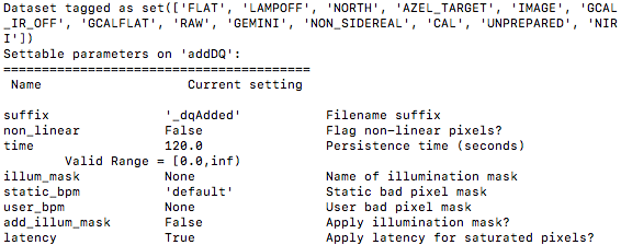
To see the list of available input parameters and their defaults, use the command line tool showpars from a terminal. It needs the name of a file on which the primitive will be run because the defaults are adjusted to match the input data.

showpars ../playdata/example1/N20160102S0363.fits addDQ

4.3.7. Standard Star

The standard star is reduced more or less the same way as the science target (next section) except that dark frames are not obtained for standard star observations. Therefore the dark correction needs to be turned off.

The processed flat field that we added earlier to the local calibration database will be fetched automatically. The user BPM (optional, but recommended) needs to be specified by the user.

reduce_std = Reduce()
reduce_std.files.extend(stdstar)
reduce_std.uparms = [('addDQ:user_bpm', bpm)]
reduce_std.uparms.append(('darkCorrect:do_cal', 'skip'))
reduce_std.runr()

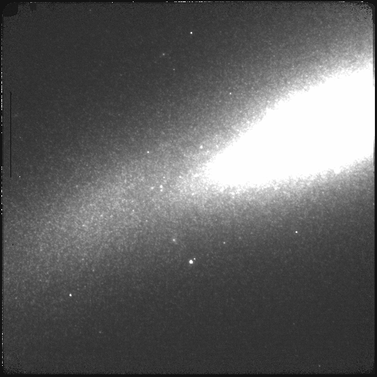
4.3.8. Science Observations

The science target is an extended source. We need to turn off the scaling of the sky because the target fills the field of view and does not represent a reasonable sky background. If scaling is not turned off in this particular case, it results in an over-subtraction of the sky frame.

The sky frame comes from off-target sky observations. We feed the pipeline all the on-target and off-target frames. The software will split the on-target and the off-target appropriately.

The master dark and the master flat will be retrieved automatically from the local calibration database. Again, the user BPM needs to be specified as the user_bpm argument to addDQ. (The static BPM will be picked from database).

The output stack units are in electrons (header keyword BUNIT=electrons). The output stack is stored in a multi-extension FITS (MEF) file. The science signal is in the “SCI” extension, the variance is in the “VAR” extension, and the data quality plane (mask) is in the “DQ” extension.

reduce_target = Reduce()
reduce_target.files.extend(target)
reduce_target.uparms = [('addDQ:user_bpm', bpm)]
reduce_target.uparms.append(('skyCorrect:scale_sky', False))
reduce_target.runr()

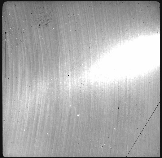
The attentive reader will note that the reduced image is slightly larger than the individual raw image. This is because of the telescope was dithered between each observation leading to a slightly larger final field of view than that of each individual image. The stacked product is not cropped to the common area, rather the image size is adjusted to include the complete area covered by the whole sequence. Of course the areas covered by less than the full stack of images will have a lower signal-to-noise.