3.3. Example 1 - Crowded with offset to sky - Using the “Reduce” class

There may be cases where you might be interested in accessing the DRAGONS’ Application Program Interface (API) directly instead of using the command line wrappers to reduce your data. In this case, you will need to access DRAGONS’ tools by importing the appropriate modules and packages.

3.3.1. The dataset

If you have not already, download and unpack the tutorial’s data package. Refer to Downloading the tutorial datasets for the links and simple instructions.

The dataset specific to this example is described in:

Example 1 - Datasets descriptions.

Here is a copy of the table for quick reference.

Science	S20170505S0095-110	Kshort-band, on target, 60 s
Flats	S20170505S0030-044 S20170505S0060-074	Lamp on, Kshort, for science Lamp off, Kshort, for science
Standard star	S20170504S0114-117	Kshort, standard star, 30 s
BMP	bpm_20121104_gsaoi_gsaoi_11_full_4amp.fits

Note

A master dark is not needed for GSAOI. The dark current is very low.

3.3.2. Setting up

First, navigate to your work directory in the unpacked data package.

cd <path>/gsaoiim_tutorial/playground

The first steps are to import libraries, set up the calibration manager, and set the logger.

3.3.2.1. Importing Libraries

We first import the necessary modules and classes:

import glob

import astrodata
import gemini_instruments
from gempy.adlibrary import dataselect
from recipe_system.reduction.coreReduce import Reduce

The dataselect module will be used to create file lists for the biases, the flats, the arcs, the standard, and the science observations. The Reduce class is used to set up and run the data reduction.

3.3.2.2. Setting up the logger

We recommend using the DRAGONS logger. (See also Double messaging issue.)

from gempy.utils import logutils
logutils.config(file_name='gsaoi_data_reduction.log')

3.3.2.3. Setting up the Calibration Service

Important

Remember to set up the calibration service.

Instructions to configure and use the calibration service are found in Setting up the Calibration Service, specifically the these sections: The Configuration File and Usage from the API.

3.3.3. Create list of files

The next step is to create input file lists. The module dataselect helps with that. It uses Astrodata tags and descriptors to select the files and store the filenames to a Python list that can then be fed to the Reduce class. (See the Astrodata User Manual for information about Astrodata and for a list of descriptors.)

The first list we create is a list of all the files in the playdata/example1 directory.

all_files = glob.glob('../playdata/example1/*.fits')
all_files.sort()

The sort() method simply re-organize the list with the file names and is an optional, but arecommended step. Before you carry on, you might want to do print(all_files) to check if they were properly read.

We will search that list for files with specific characteristics. We use the all_files list as an input to the function dataselect.select_data() . The function’s signature is:

select_data(inputs, tags=[], xtags=[], expression='True')

We show several usage examples below.

3.3.3.1. A list for the flats

Now you must create a list of FLAT images for each filter. The expression specifying the filter name is needed only if you have data from multiple filters. It is not really needed in this case.

list_of_flats_Ks = dataselect.select_data(
     all_files,
     ['FLAT'],
     [],
     dataselect.expr_parser('filter_name=="Kshort"')
)

3.3.3.2. A list for the standard star

For the standard star selection, we use:

list_of_std_stars = dataselect.select_data(
    all_files,
    [],
    [],
    dataselect.expr_parser('observation_class=="partnerCal"')
)

Here, we are passing empty lists to the second and the third argument since we do not need to use the Tags for selection nor for exclusion.

3.3.3.3. A list for the science data

Finally, the science data can be selected using:

list_of_science_images = dataselect.select_data(
    all_files,
    [],
    [],
    dataselect.expr_parser('(observation_class=="science" and exposure_time==60.)')
)

The exposure time is not really needed in this case since there are only 60-second frames, but it shows how you could have two selection criteria in the expression.

3.3.4. Bad Pixel Mask

Starting with DRAGONS v3.1, the static bad pixel masks (BPMs) are now handled as calibrations. They are downloadable from the archive instead of being packaged with the software. They are automatically associated like any other calibrations. This means that the user now must download the BPMs along with the other calibrations and add the BPMs to the local calibration manager.

See Getting Bad Pixel Masks from the archive in Tips and Tricks to learn about the various ways to get the BPMs from the archive.

To add the BPM included in the data package to the local calibration database:

for bpm in dataselect.select_data(all_files, ['BPM']):
    caldb.add_cal(bpm)

3.3.5. Create a Master Flat Field

As explained on the calibration webpage for GSAOI, dark subtraction is not necessary since the dark noise level is very low. Therefore, we can go ahead and start with the master flat.

A GSAOI K-short master flat is created from a series of lamp-on and lamp-off exposures. Each flavor is stacked, then the lamp-off stack is subtracted from the lamp-on stack and the result normalized.

We create the master flat field and add it to the calibration manager as follow:

reduce_flats = Reduce()
reduce_flats.files.extend(list_of_flats_Ks)
reduce_flats.runr()

Note

The file name of the output processed flat is the file name of the first file in the list with _flat appended as a suffix. This is the general naming scheme used by the Recipe System.

Note

If you wish to inspect the processed calibrations before adding them to the calibration database, remove the “store” option attached to the database in the dragonsrc configuration file. You will then have to add the calibrations manually following your inspection, eg.

caldb.add_cal(reduce_flats.output_filenames[0])

3.3.6. Reduce Standard Star

The standard star is reduced essentially the same way as the science target (next section). The processed flat field that we added above to the local calibration database will be fetched automatically.

reduce_std = Reduce()
reduce_std.files.extend(list_of_std_stars)
reduce_std.runr()

Note

Reduce will automatically align and stack the images. Therefore, it is no longer necessary to use the disco_stu tool for GSAOI data.

3.3.7. Reduce the Science Images

The science observation uses a dither-on-target with offset-to-sky pattern. The sky frames from the offset-to-sky position will be automatically detected and used for the sky subtraction.

The BPM and the master flat will be retrieved automatically from the local calibration database.

We use similar commands as before to initiate a new reduction to reduce the science data:

reduce_target = Reduce()
reduce_target.files.extend(list_of_science_images)
reduce_target.uparms.append(('skyCorrect:offset_sky', False))
reduce_target.runr()

This will generate flat corrected files, align them, stack them, and orient them such that North is up and East is left. The final image will have the name of the first file in the set, with the suffix _image. The on-target files are the ones that have been flat corrected (_flatCorrected), and scaled (_countsScaled). There should be nine of these.

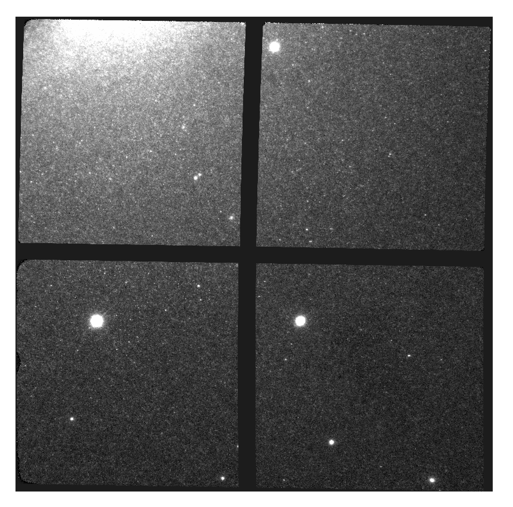
S20170505S0095 - Final flat corrected, aligned, and stacked image

The figure above shows the final flat-corrected, aligned, and stacked frame. For absolute distortion correction and astrometry, Reduce can use a reference catalog provided by the user. Without a reference catalog, like above, only the relative distortion between the frames is accounted for.

The output stack units are in electrons (header keyword BUNIT=electrons). The output stack is stored in a multi-extension FITS (MEF) file. The science signal is in the “SCI” extension, the variance is in the “VAR” extension, and the data quality plane (mask) is in the “DQ” extension.