4.3. Example 2 - Separate CCDs - Using the “Reduce” class
A reduction can be initiated from the command line as shown in Example 2 - Separate CCDs - Using the “reduce” command line and it can also be done programmatically as we will show here. The classes and modules of the RecipeSystem can be accessed directly for those who want to write Python programs to drive their reduction. In this example we replicate the command line version of Example 2 but using the Python programmatic interface. What is shown here could be packaged in modules for greater automation.
Instead of running the default recipe, we will run the recipe to reduce the CCDs separately instead of mosaicing them before the stack. Doing the reduction this way and not mosaicing the CCDs is used when the science objective require very accurate photometry that needs to take into account color-terms and the different color responses of the CCDs.
4.3.1. The dataset
If you have not already, download and unpack the tutorial’s data package. Refer to Downloading the tutorial datasets for the links and simple instructions.
The dataset specific to this example is described in:
Here is a copy of the table for quick reference.
Science |
N20220627S0115-119
|
350 s, i-band
|
Bias |
N20220613S0180-184
N20220627S0222-226
|
For science
For twilights
|
Twilight Flats |
N20220613S0138-142
|
r-band
|
BPM |
bpm_20220303_gmos-n_Ham_22_full_12amp.fits
|
|
4.3.2. Setting Up
4.3.2.1. Importing Libraries
We first import the necessary modules and classes:
1import glob
2
3import astrodata
4import gemini_instruments
5from recipe_system.reduction.coreReduce import Reduce
6from gempy.adlibrary import dataselect
The dataselect module will be used to create file lists for the
biases, the flats, the arcs, the standard, and the science observations.
The Reduce class is used to set up and run the data
reduction.
4.3.2.2. Setting up the logger
We recommend using the DRAGONS logger. (See also Double messaging issue.)
7from gempy.utils import logutils
8logutils.config(file_name='gmos_data_reduction.log')
4.3.2.3. Setting up the Calibration Service
Important
Remember to set up the calibration service.
Instructions to configure and use the calibration service are found in Setting up the Calibration Service, specifically the these sections: The Configuration File and Usage from the API.
4.3.3. Create list of files
The next step is to create input file lists. The module dataselect helps
with that. It uses Astrodata tags and descriptors to select the files and
store the filenames to a Python list that can then be fed to the Reduce
class. (See the Astrodata User Manual for information about Astrodata and for a list
of descriptors.)
The first list we create is a list of all the files in the playdata/example2/
directory.
 9all_files = glob.glob('../playdata/example2/*.fits')
10all_files.sort()
The sort() method simply re-organize the list with the file names
and is an optional step, but a recommended step. Before you carry on, you
might want to do print(all_files) to check if they were properly read.
We will search that list for files with specific characteristics. We use
the all_files list as an input to the function
dataselect.select_data() . The function’s signature is:
select_data(inputs, tags=[], xtags=[], expression='True')
We show several usage examples below.
4.3.3.1. List of Biases
We are going to use two sets of biases, one for the science and one for the twilights. The reason for that is that the twilights and the science were obtained weeks apart and it is always safer to use biases that were obtained close in time with the data we want to use them on. It is also a good example to show you how to specify a date range in the dataselect expression.
The command line showd can be used to inspect the data ahead of time.
$ showd -d object,ut_date ../playdata/example2/N*.fits

  --------------------------------------------------------------------------------
  filename                                                     object      ut_date
  --------------------------------------------------------------------------------
  ../playdata/example2/N20220613S0138.fits                   Twilight   2022-06-13
  ../playdata/example2/N20220613S0139.fits                   Twilight   2022-06-13
  ../playdata/example2/N20220613S0140.fits                   Twilight   2022-06-13
  ../playdata/example2/N20220613S0141.fits                   Twilight   2022-06-13
  ../playdata/example2/N20220613S0142.fits                   Twilight   2022-06-13
  ../playdata/example2/N20220613S0180.fits                       Bias   2022-06-13
  ../playdata/example2/N20220613S0181.fits                       Bias   2022-06-13
  ../playdata/example2/N20220613S0182.fits                       Bias   2022-06-13
  ../playdata/example2/N20220613S0183.fits                       Bias   2022-06-13
  ../playdata/example2/N20220613S0184.fits                       Bias   2022-06-13
  ../playdata/example2/N20220627S0115.fits   Disrupting UFD Candidate   2022-06-27
  ../playdata/example2/N20220627S0116.fits   Disrupting UFD Candidate   2022-06-27
  ../playdata/example2/N20220627S0117.fits   Disrupting UFD Candidate   2022-06-27
  ../playdata/example2/N20220627S0118.fits   Disrupting UFD Candidate   2022-06-27
  ../playdata/example2/N20220627S0119.fits   Disrupting UFD Candidate   2022-06-27
  ../playdata/example2/N20220627S0222.fits                       Bias   2022-06-27
  ../playdata/example2/N20220627S0223.fits                       Bias   2022-06-27
  ../playdata/example2/N20220627S0224.fits                       Bias   2022-06-27
  ../playdata/example2/N20220627S0225.fits                       Bias   2022-06-27
  ../playdata/example2/N20220627S0226.fits                       Bias   2022-06-27
The science frames were obtained on 2022-06-27 and the twilights on 2022-06-13. We will create two lists, one of the biases obtained on each of those two days.
Let us select the files that will be used to create the two master biases:
11list_of_biastwi = dataselect.select_data(
12    all_files,
13    ['BIAS'],
14    [],
15    dataselect.expr_parser("ut_date=='2022-06-13'")
16)
17
18list_of_biassci = dataselect.select_data(
19    all_files,
20    ['BIAS'],
21    [],
22    dataselect.expr_parser("ut_date=='2022-06-27'")
23)
4.3.3.2. List of Flats
Next we create a list of twilight flats for each filter. The expression specifying the filter name is needed only if you have data from multiple filters. It is not really needed in this case.
24list_of_flats = dataselect.select_data(
25    all_files,
26    ['FLAT'],
27    [],
28    dataselect.expr_parser('filter_name=="r"')
29)
Note
All expressions need to be processed with dataselect.expr_parser.
4.3.3.3. List of Science Data
Finally, the science data can be selected using:
30list_of_science = dataselect.select_data(
31    all_files,
32    [],
33    ['CAL'],
34    dataselect.expr_parser('(observation_class=="science" and filter_name=="r")')
35)
Here we left the tags argument as an empty list and passed the tag
'CAL' as an exclusion tag through the xtags argument.
We also added a fourth argument which is not necessary for our current dataset
but that can be useful for others. It contains an expression that has to be
parsed by dataselect.expr_parser, and which ensures
that we are getting science frames obtained with the r-band filter.
4.3.4. Bad Pixel Mask
Starting with DRAGONS v3.1, the static bad pixel masks (BPMs) are now handled as calibrations. They are downloadable from the archive instead of being packaged with the software. They are automatically associated like any other calibrations. This means that the user now must download the BPMs along with the other calibrations and add the BPMs to the local calibration manager.
See Getting Bad Pixel Masks from the archive in Tips and Tricks to learn about the various ways to get the BPMs from the archive.
To add the BPM included in the data package to the local calibration database:
36for bpm in dataselect.select_data(all_files, ['BPM']):
37    caldb.add_cal(bpm)
4.3.5. Make Master Bias
The reduction of the biases does not mosaic the biases and it keeps the CCDs separated, always. Because of that, the reduction of the biases for the “Separate CCDs” recipe is exactly the same as for the default recipe.
We create the master bias and add it to the calibration manager as follows:
38reduce_biastwi = Reduce()
39reduce_biastwi.files.extend(list_of_biastwi)
40reduce_biastwi.runr()
41
42reduce_biassci = Reduce()
43reduce_biassci.files.extend(list_of_biassci)
44reduce_biassci.runr()
The Reduce class is our reduction
“controller”. This is where we collect all the information necessary for
the reduction. In this case, the only information necessary is the list of
input files which we add to the files attribute. The
Reduce.runr method is where the
recipe search is triggered and where it is executed.
Note
The file name of the output processed bias is the file name of the
first file in the list with _bias appended as a suffix. This is the
general naming scheme used by the Recipe System.
Note
If you wish to inspect the processed calibrations before adding them
to the calibration database, remove the “store” option attached to the
database in the dragonsrc configuration file. You will then have to
add the calibrations manually following your inspection, eg.
caldb.add_cal(reduce_biassci.output_filenames[0])
4.3.6. Make Master Flat
The reduction of the flats does not mosaic the flats and it keeps the CCDs separated, always. Because of that, the reduction of the flats for the “Separate CCDs” recipe is exactly the same as for the default recipe.
We create the master flat field and add it to the calibration database as follows:
45reduce_flats = Reduce()
46reduce_flats.files.extend(list_of_flats)
47reduce_flats.runr()
4.3.7. Make Master Fringe Frame
Warning
The dataset used in this tutorial does not require fringe correction so we skip this step. To find out how to produce a master fringe frame, see Create Master Fringe Frame in the Tips and Tricks chapter.
4.3.8. Reduce Science Images
We use similar statements as before to initiate a new reduction to reduce the
science data. Instead of using the default recipe, we
will explicitly call the recipe reduceSeparateCCDs:
48reduce_science = Reduce()
49reduce_science.files.extend(list_of_science)
50reduce_science.recipename = 'reduceSeparateCCDs'
51reduce_science.runr()
This recipe performs the standardization and corrections needed to convert the raw input science images into a stacked image. To deal with different color terms on the different CCDs, the images are split by CCD midway through the recipe and subsequently reduced separately. The relative WCS is determined from mosaicked versions of the images and then applied to each of the CCDs separately.
The stacked images of each CCD are in separate extension of the file
with the _image suffix.
When you display the image, you will notice that some sources appear on two CCDs. This is because the each CCD has been stacked individually and because of the dithers some sources ended up moving from to the adjacent CCD.
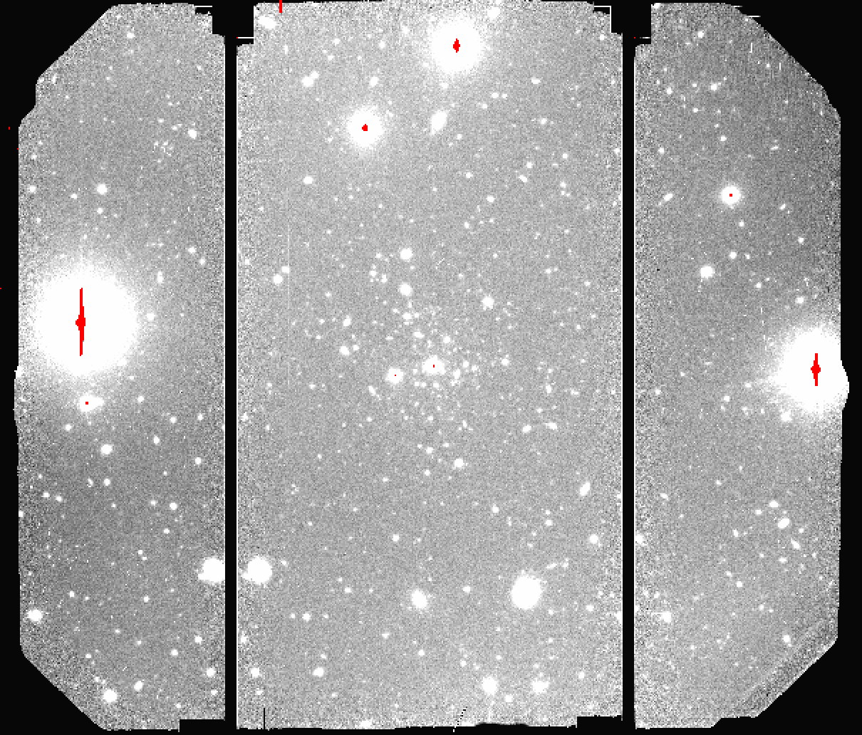
Final stacked image, with CCD separated.
The output stack units are in electrons (header keyword BUNIT=electrons). The output stack is stored in a multi-extension FITS (MEF) file. The science signal is in the “SCI” extension, the variance is in the “VAR” extension, and the data quality plane (mask) is in the “DQ” extension.
Note
There is another similar recipe that can be used to reduce the CCDs
separately: reduceSeparateCCDsCentral. The difference is that
the relative WCS is determined from the central CCD
(CCD2) and then applied to CCDs 1 and 3, while in reduceSeparateCCDs
the whole image is used to adjust the WCS. The “Central” recipe can be
faster than the other but potentially less accurate if you do not have
a lot of sources in CCD2.