4.3. Example 2 - Deep observation - Using the “Reduce” class
There may be cases where you would be interested in accessing the DRAGONS Application Program Interface (API) directly instead of using the command line wrappers to reduce your data. Here we show you how to do the same reduction we did in the previous chapter, Example 2 - Deep observation - Using the “reduce” command line, but using the API.
4.3.1. The dataset
If you have not already, download and unpack the tutorial’s data package. Refer to Downloading the tutorial datasets for the links and simple instructions.
The dataset specific to this example is described in:
Here is a copy of the table for quick reference.
Science |
S20200104S0075-092
|
K-red, 5 s |
Darks |
S20200107S0035-041
S20200111S0257-260
|
2 s, darks for flats 2 s, darks for flats |
S20200107S0049-161
|
5 s, for science dat |
|
Flats |
S20200108S0010-019
|
2 s, Lamp On, K-red |
4.3.2. Setting Up
First, navigate to your work directory in the unpacked data package.
cd <path>/f2im_tutorial/playground
The first steps are to import libraries, set up the calibration manager, and set the logger.
4.3.2.1. Importing Libraries
We first import the necessary modules and classes:
1import glob
2
3import astrodata
4import gemini_instruments
5from recipe_system.reduction.coreReduce import Reduce
6from gempy.adlibrary import dataselect
The dataselect module will be used to create file lists for the
biases, the flats, the arcs, the standard, and the science observations.
The Reduce class is used to set up and run the data
reduction.
4.3.2.2. Setting up the logger
We recommend using the DRAGONS logger. (See also Double messaging issue.)
7from gempy.utils import logutils
8logutils.config(file_name='f2im_data_reduction.log')
4.3.2.3. Setting up the Calibration Service
Important
Remember to set up the calibration service.
Instructions to configure and use the calibration service are found in Setting up the Calibration Service, specifically the these sections: The Configuration File and Usage from the API.
4.3.3. Create list of files
The next step is to create input file lists. The module dataselect helps
with that. It uses Astrodata tags and descriptors to select the files and
store the filenames to a Python list that can then be fed to the Reduce
class. (See the Astrodata User Manual for information about Astrodata and for a list
of descriptors.)
The first list we create is a list of all the files in the playdata/example2/
directory.
 9all_files = glob.glob('../playdata/example2/*.fits')
10all_files.sort()
The sort() method simply re-organize the list with the file names
and is an optional, but a recommended step. Before you carry on, you might want to do
print(all_files) to check if they were properly read.
We will search that list for files with specific characteristics. We use
the all_files list as an input to the function
dataselect.select_data() . The function’s signature is:
select_data(inputs, tags=[], xtags=[], expression='True')
We show several usage examples below.
4.3.3.1. Two lists for the darks
We select the files that will be used to create a master dark for the science observations, those with an exposure time of 5 seconds.
11dark_files_5s = dataselect.select_data(
12    all_files,
13    ['F2', 'DARK', 'RAW'],
14    [],
15    dataselect.expr_parser('exposure_time==5')
16)
Above we are requesting data with tags F2, DARK, and RAW, though
since we only have F2 raw data in the directory, DARK would be sufficient
in this case. We are not excluding any tags, as represented by the empty
list [].
Note
All expressions need to be processed with dataselect.expr_parser.
We repeat the same syntax for the 2-second darks:
17dark_files_2s = dataselect.select_data(
18    all_files,
19    ['F2', 'DARK', 'RAW'],
20    [],
21    dataselect.expr_parser('exposure_time==2')
22)
4.3.3.2. A list for the flats
Now you must create a list of FLAT images for each filter. The expression specifying the filter name is needed only if you have data from multiple filters. It is not really needed in this case.
23list_of_flats_Kred = dataselect.select_data(
24     all_files,
25     ['FLAT'],
26     [],
27     dataselect.expr_parser('filter_name=="K-red"')
28)
4.3.3.3. A list for the science data
Finally, the science data can be selected using:
29list_of_science_images = dataselect.select_data(
30    all_files,
31    ['F2'],
32    [],
33    dataselect.expr_parser('(observation_class=="science" and filter_name=="K-red")')
34)
The filter name is not really needed in this case since there are only Y-band frames, but it shows how you could have two selection criteria in the expression.
4.3.4. Create a Master Dark
We first create the master dark for the science targe.The master biases
will be automatically added to the local calibration manager when the “store”
parameter is present in the .dragonsrc configuration file.
The name of the output master dark is
S20200107S0049_dark.fits. The output is written to disk and its name is
stored in the Reduce instance. The calibration service expects the name of a
file on disk.
35reduce_darks = Reduce()
36reduce_darks.files.extend(dark_files_5s)
37reduce_darks.runr()
The Reduce class is our reduction
“controller”. This is where we collect all the information necessary for
the reduction. In this case, the only information necessary is the list of
input files which we add to the files attribute. The runr method is
where the recipe search is triggered and where it is executed.
Note
The file name of the output processed dark is the file name of the
first file in the list with _dark appended as a suffix. This is the general
naming scheme used by the Recipe System.
Note
- If you wish to inspect the processed calibrations before adding them
to the calibration database, remove the “store” option attached to the database in the
dragonsrcconfiguration file. You will then have to add the calibrations manually following your inspection, eg.
caldb.add_cal(reduce_darks.output_filenames[0])
4.3.5. Create a Master Flat Field
The F2 K-red master flat is created from a series of lamp-off exposures and darks. They should all have the same exposure time. Each flavor is stacked (averaged), then the dark stack is subtracted from the lamp-off stack and the result normalized.
We create the master flat field and add it to the calibration manager as follows:
38reduce_flats = Reduce()
39reduce_flats.files.extend(list_of_flats_Kred)
40reduce_flats.files.extend(dark_files_2s)
41reduce_flats.runr()
It is important to put the flats first in that call. The recipe is selected based on the astrodata tags of the first file in the list of inputs.
4.3.6. Reduce the Science Images
The science observation uses a dither-on-target pattern. The sky frames will be derived automatically for each science frame from the dithered frames.
The master dark and the master flat will be retrieved automatically from the local calibration database.
We will be running the ultradeep recipe, the 3-part version. If you
prefer to run the whole thing in one shot, just call the full recipe with
reduce_target.recipename = 'ultradeep'.
The first part of the ultradeep recipe does the pre-processing, up to and including the flatfield correction. This part is identical to what is being done the in default F2 recipe.
42reduce_target = Reduce()
43reduce_target.files = list_of_science_images
44reduce_target.recipename = 'ultradeep_part1'
45reduce_target.runr()
The outputs are the _flatCorrected files. The list is stored in
reduce_target.output_filenames which we can pass to the next call.
The ultradeep_part2 recipe takes _flatCorrected images from part 1 as
input and continues the reduction to produce a stacked image. It then
identifies sources in the stack and transfers the object mask (OBJMASK) back
to the individual input images, saving those to disk, ready for part 3.
46reduce_target.files = reduce_target.output_filenames
47reduce_target.recipename = 'ultradeep_part2'
48reduce_target.runr()
The outputs are the _objmaskTransferred files.
Finally, the ultradeep_part3 recipe takes flat-corrected images with
the object masks (_objmaskTransferred) as inputs and produces a final stack.
49reduce_target.files = reduce_target.output_filenames
50reduce_target.recipename = 'ultradeep_part3'
51reduce_target.runr()
The final product file will have a _image.fits suffix.
The output stack units are in electrons (header keyword BUNIT=electrons). The output stack is stored in a multi-extension FITS (MEF) file. The science signal is in the “SCI” extension, the variance is in the “VAR” extension, and the data quality plane (mask) is in the “DQ” extension.
For this dataset the benefit of the ultradeep recipe is subtle. Below we show a zoomed-in section of the final image when the complete set of 156 images is used. The image on the left is from the default recipe, the one on the right is from the ultradeep recipe.
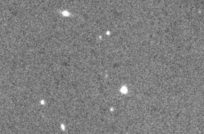
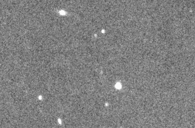
Looking very carefully, it is possible to see weak blotching in the default recipe image (left) that does dissappear when the ultradeep recipe is used. Even using the full set, it is still subtle. Therefore, we recommend the use of the ultradeep recipe only when you actually needed or when the blotching is more severe. The blotching is expected to be more severe in crowded fields.