3.2. Example 1 - Small sources with dither on target - Using the “reduce” command line
This chapter will guide you on reducing Flamingos-2 imaging data using command line tools. In this example we reduce a Flamingos-2 observation of a star and distant galaxy field. The observation is a simple dither-on-target sequence. Just open a terminal to get started.
While the example cannot possibly cover all situations, it will help you get acquainted with the reduction of Flamingos-2 data with DRAGONS. We encourage you to look at the Tips and Tricks and Issues and Limitations chapters to learn more about F2 data reduction.
DRAGONS installation comes with a set of useful scripts that are used to reduce astronomical data. The most important script is called reduce, which is extensively explained in the Recipe System Users Manual. It is through that command that a DRAGONS reduction is launched.
For this tutorial, we will be also using other support tools like:
3.2.1. The dataset
If you have not already, download and unpack the tutorial’s data package. Refer to Downloading the tutorial datasets for the links and simple instructions.
The dataset specific to this example is described in:
Here is a copy of the table for quick reference.
Science |
S20131121S0075-083
|
Y-band, 120 s |
Darks |
S20131121S0369-375
|
2 s, short darks for BPM |
S20131120S0115-120
S20131121S0010
S20131122S0012
S20131122S0438-439
|
120 s, for science data |
|
Flats |
S20131129S0320-323
|
20 s, Lamp On, Y-band |
S20131126S1111-116
|
20 s, Lamp Off, Y-band |
3.2.2. Set up the Calibration Service
Important
Remember to set up the calibration service.
Instructions to configure and use the calibration service are found in Setting up the Calibration Service, specifically the these sections: The Configuration File and Usage from the Command Line.
3.2.3. Check files
For this example, all the raw files we need are in the same directory called
../playdata/example1/. Let us learn a bit about the data we have.
Ensure that you are in the playground directory and that the conda
environment that includes DRAGONS has been activated.
Let us call the command tool typewalk:
$ typewalk -d ../playdata/example1/

directory:  /path_to_my_files/f2img_tutorial/playdata/example1
     S20131120S0115.fits ............... (AT_ZENITH) (AZEL_TARGET) (CAL) (DARK) (F2) (GEMINI) (NON_SIDEREAL) (RAW) (SOUTH) (UNPREPARED)
     ...
     S20131121S0075.fits ............... (F2) (GEMINI) (IMAGE) (RAW) (SIDEREAL) (SOUTH) (UNPREPARED)
     ...
     S20131121S0369.fits ............... (AT_ZENITH) (AZEL_TARGET) (CAL) (DARK) (F2) (GEMINI) (NON_SIDEREAL) (RAW) (SOUTH) (UNPREPARED)
     ...
     S20131126S1111.fits ............... (AZEL_TARGET) (CAL) (F2) (FLAT) (GCALFLAT) (GCAL_IR_OFF) (GEMINI) (IMAGE) (LAMPOFF) (NON_SIDEREAL) (RAW) (SOUTH) (UNPREPARED)
     ...
     S20131129S0320.fits ............... (AT_ZENITH) (AZEL_TARGET) (CAL) (F2) (FLAT) (GCALFLAT) (GCAL_IR_ON) (GEMINI) (IMAGE) (LAMPON) (NON_SIDEREAL) (RAW) (SOUTH) (UNPREPARED)
     ...
Done DataSpider.typewalk(..)
This command will open every FITS file within the directory passed after the -d
flag (recursively) and will print an unsorted table with the file names and the
associated tags. For example, calibration files will always have the CAL
tag. Flat images will always have the FLAT tag. Dark files will have the
DARK tag. This means that we can start getting to know a bit more about our
data set just by looking at the tags. The output above was trimmed for
presentation.
3.2.4. Create file lists
This data set contains science and calibration frames. For some programs, it could have different observed targets and different exposure times depending on how you like to organize your raw data.
The DRAGONS data reduction pipeline does not organize the data for you. You have to do it. DRAGONS provides tools to help you with that.
The first step is to create input file lists. The tool “dataselect” helps with that. It uses Astrodata tags and “descriptors” to select the files and send the filenames to a text file that can then be fed to “reduce”. (See the Astrodata User Manual for information about Astrodata.)
First, navigate to the playground directory in the unpacked data package:
cd <path>/f2im_tutorial/playground
3.2.4.1. Two lists for the darks
Our data set contains two sets of DARK files: some 120-second darks matching the science data and some 2-second darks to create the bad pixel mask (BPM). If you did not know the exposure times of the darks, you could send the dataselect results to the showd command line tool as follows to get the information:
$ dataselect --tags DARK ../playdata/example1/*.fits | showd -d exposure_time
--------------------------------------------------------
filename                                   exposure_time
--------------------------------------------------------
../playdata/example1/S20131120S0115.fits           120.0
../playdata/example1/S20131120S0116.fits           120.0
../playdata/example1/S20131120S0117.fits           120.0
...
../playdata/example1/S20131121S0369.fits             2.0
../playdata/example1/S20131121S0370.fits             2.0
../playdata/example1/S20131121S0371.fits             2.0
...
../playdata/example1/S20131122S0012.fits           120.0
../playdata/example1/S20131122S0438.fits           120.0
../playdata/example1/S20131122S0439.fits           120.0
(The list has been shortened for presentation.)
The | is the Unix “pipe” operator and it is used to pass output from
dataselect to showd.
Let us go ahead and create our two list of darks. The following line creates a list of dark files that have exposure time of 120 seconds:
$ dataselect --tags DARK --expr "exposure_time==120" ../playdata/example1/*.fits -o darks_120s.list
--expr is used to filter the files based on their descriptors. Here we are
selecting files with exposure time of 120 seconds. You can repeat the same
command with the other exposure time to get the list of short darks.
$ dataselect --tags DARK --expr "exposure_time==2" ../playdata/example1/*.fits -o darks_002s.list
3.2.4.2. A list for the flats
Now let us create the list containing the flat files:
$ dataselect --tags FLAT ../playdata/example1/*.fits -o flats.list
We know that our dataset has only one filter (Y-band). If our dataset
contained data with more filters, we would have had to use the --expr
option to select the appropriate filter as follows:
$ dataselect --tags FLAT --expr "filter_name=='Y'" ../playdata/example1/*.fits -o flats_Y.list
Note
Flamingos-2 Y, J and H flat fields are created from lamps-on and lamps-off flats. The software will sort them out, so put all lamps-on, lamp-off flats, in the list and let the software use them appropriately.
3.2.4.3. A list for the science observations
Finally, we want to create a list of the science targets. We are looking for
files that are not calibration frames. To exclude them from our
selection we can use the --xtags, e.g., --xtags CAL.
$ dataselect --xtags CAL ../playdata/example1/*.fits -o sci_images.list
Remember that you can use the --expr option to select targets with different
names (object) or exposure times (exposure_time), or use it with any
of the datasets descriptors.
3.2.5. Create a Master Dark
We start the data reduction by creating a master dark for the science data. Here is how you reduce the 120 s dark data into a master dark:
$ reduce @darks_120s.list
The @ character before the name of the input file is the “at-file” syntax.
More details can be found in the "at-file" Facility documentation.
Because the database was given the “store” option in the dragonsrc file,
the processed dark will be automatically added to the database at the end of
the recipe.
Note
The file name of the output processed dark is the file name of the
first file in the list with _dark appended as a suffix. This the
general naming scheme used by “reduce”.
Note
If you wish to inspect the processed calibrations before adding them
to the calibration database, remove the “store” option attached to the
database in the dragonsrc configuration file. You will then have to
add the calibrations manually following your inspection, eg.
caldb add S20131120S0115_dark.fits
Note
The master dark will be saved in the same folder where reduce was
called and inside the ./calibrations/processed_dark folder. The latter
location is to cache a copy of the file. This applies to all the processed
calibration.
3.2.6. Create a Bad Pixel Mask
A Bad Pixel Mask (BPM) can be built using a set of flat images with the lamps on and off and a set of short exposure dark files. Here, our shortest dark files have 2 second exposure time. Again, we use the reduce command to produce the BPMs.
It is important to note that the recipe library association is done based on the nature of the first file in the input list. Since the recipe to make the BPM is located in the recipe library for flats, the first item in the list must be a flat.
For Flamingos-2, the filter wheel’s location is such that the choice of filter does not interfere with the results. Here we have Y-band flats, so we will use Y-band flats.
$ reduce @flats_Y.list @darks_002s.list -r makeProcessedBPM
The -r tells reduce which recipe from the recipe library for F2-FLAT
to use. If not specified the system will use the default recipe which is the
one that produces a master flat, this is not what we want here. The output
image will be saved in the current working directory with a _bpm suffix.
Since this is a user-made BPM, you will have to pass it to DRAGONS on the as an option on the command line.
3.2.7. Create a Master Flat Field
The F2 Y-band master flat is created from a series of lamp-on and lamp-off exposures. They should all have the same exposure time. Each flavor is stacked (averaged), then the lamp-off stack is subtracted from the lamp-on stack and the result normalized.
We create the master flat field and add it to the calibration manager as follow:
$ reduce @flats_Y.list -p addDQ:user_bpm="S20131129S0320_bpm.fits"
Here, the -p flag tells reduce to set the input parameter user_bpm
of the addDQ primitive to the filename of the BPM we have just created.
There will be a message “WARNING - No static BPMs defined”. This is
normal. This is because F2 does not have a static BPM that is distributed
with the associated calibrations. Your user BPM is the only one that is
available.
3.2.8. Reduce the Science Images
Now that we have the master dark and the master flat, we can tell reduce to process our science data. reduce will look at the local database for calibration files.
$ reduce @sci_images.list -p addDQ:user_bpm="S20131129S0320_bpm.fits"
This command retrieves the master dark and the master flat, and applies them to the science data. For sky subtraction, the software analyses the sequence to establish whether this is a dither-on-target or an offset-to-sky sequence and then proceeds accordingly. Finally, the sky-subtracted frames are aligned and stacked together. Sources in the frames are used for the alignment.
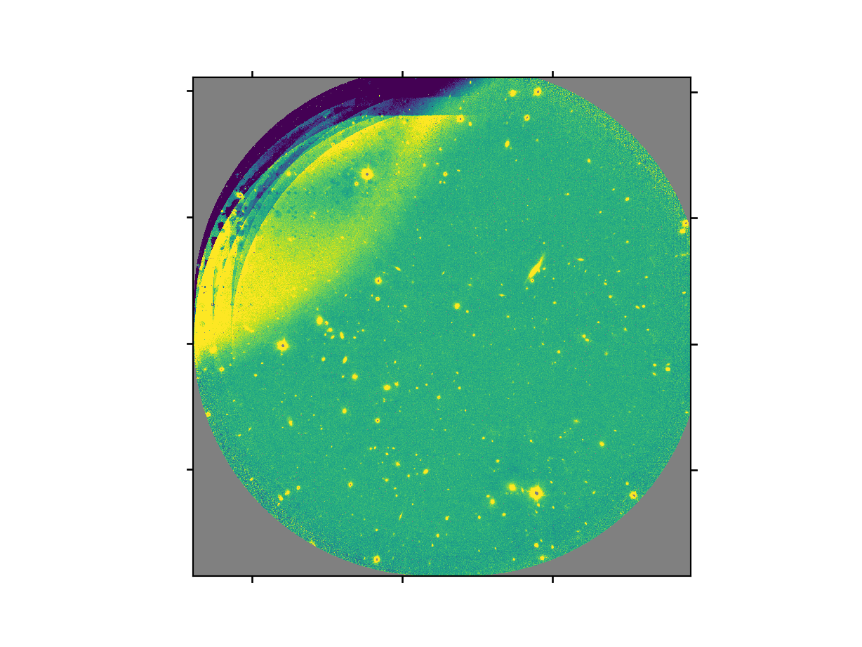
The final product file will have a _image.fits suffix and it is shown below.
The output stack units are in electrons (header keyword BUNIT=electrons). The output stack is stored in a multi-extension FITS (MEF) file. The science signal is in the “SCI” extension, the variance is in the “VAR” extension, and the data quality plane (mask) is in the “DQ” extension.
Warning
The upper-left quadrant of this science sequence is rather messy. This is caused by the PWFS2 guide probe (see Emission from PWFS2 guide probe). Photometry in this portion of the image is likely to be seriously compromised.