3.3. Example 1 - Small sources with dither on target - Using the “Reduce” class

There may be cases where you would be interested in accessing the DRAGONS Application Program Interface (API) directly instead of using the command line wrappers to reduce your data. Here we show you how to do the same reduction we did in the previous chapter but using the API.

3.3.1. The dataset

If you have not already, download and unpack the tutorial’s data package. Refer to Downloading the tutorial datasets for the links and simple instructions.

The dataset specific to this example is described in:

Example 1 - Datasets descriptions.

Here is a copy of the table for quick reference.

Science	S20131121S0075-083	Y-band, 120 s
Darks	S20131121S0369-375	2 s, short darks for BPM
	S20131120S0115-120 S20131121S0010 S20131122S0012 S20131122S0438-439	120 s, for science data
Flats	S20131129S0320-323	20 s, Lamp On, Y-band
	S20131126S1111-116	20 s, Lamp Off, Y-band

3.3.2. Setting Up

First, navigate to your work directory in the unpacked data package.

cd <path>/f2im_tutorial/playground

The first steps are to import libraries, set up the calibration manager, and set the logger.

3.3.2.1. Importing Libraries

We first import the necessary modules and classes:

import glob

import astrodata
import gemini_instruments
from recipe_system.reduction.coreReduce import Reduce
from gempy.adlibrary import dataselect

The dataselect module will be used to create file lists for the biases, the flats, the arcs, the standard, and the science observations. The Reduce class is used to set up and run the data reduction.

3.3.2.2. Setting up the logger

We recommend using the DRAGONS logger. (See also Double messaging issue.)

from gempy.utils import logutils
logutils.config(file_name='f2im_data_reduction.log')

3.3.2.3. Setting up the Calibration Service

Important

Remember to set up the calibration service.

Instructions to configure and use the calibration service are found in Setting up the Calibration Service, specifically the these sections: The Configuration File and Usage from the API.

3.3.3. Create list of files

The next step is to create input file lists. The module dataselect helps with that. It uses Astrodata tags and descriptors to select the files and store the filenames to a Python list that can then be fed to the Reduce class. (See the Astrodata User Manual for information about Astrodata and for a list of descriptors.)

The first list we create is a list of all the files in the playdata/example1/ directory.

all_files = glob.glob('../playdata/example1/*.fits')
all_files.sort()

The sort() method simply re-organize the list with the file names and is an optional, but a recommended step. Before you carry on, you might want to do print(all_files) to check if they were properly read.

We will search that list for files with specific characteristics. We use the all_files list as an input to the function dataselect.select_data() . The function’s signature is:

select_data(inputs, tags=[], xtags=[], expression='True')

We show several usage examples below.

3.3.3.1. Two lists for the darks

We select the files that will be used to create a master dark for the science observations, those with an exposure time of 120 seconds.

dark_files_120s = dataselect.select_data(
    all_files,
    ['F2', 'DARK', 'RAW'],
    [],
    dataselect.expr_parser('exposure_time==120')
)

Above we are requesting data with tags F2, DARK, and RAW, though since we only have F2 raw data in the directory, DARK would be sufficient in this case. We are not excluding any tags, as represented by the empty list [].

Note

All expressions need to be processed with dataselect.expr_parser.

We repeat the same syntax for the 2-second darks:

dark_files_2s = dataselect.select_data(
    all_files,
    ['F2', 'DARK', 'RAW'],
    [],
    dataselect.expr_parser('exposure_time==2')
)

3.3.3.2. A list for the flats

Now you must create a list of FLAT images for each filter. The expression specifying the filter name is needed only if you have data from multiple filters. It is not really needed in this case.

list_of_flats_Y = dataselect.select_data(
     all_files,
     ['FLAT'],
     [],
     dataselect.expr_parser('filter_name=="Y"')
)

3.3.3.3. A list for the science data

Finally, the science data can be selected using:

list_of_science_images = dataselect.select_data(
    all_files,
    ['F2'],
    [],
    dataselect.expr_parser('(observation_class=="science" and filter_name=="Y")')
)

The filter name is not really needed in this case since there are only Y-band frames, but it shows how you could have two selection criteria in the expression.

Note

For Flamingos-2 data, it is useful to check the World Coordinate System (WCS) of the science data.

checkwcs = Reduce()
checkwcs.files = list_of_science_images
checkwcs.recipename = 'checkWCS'
checkwcs.runr()

Please see details in Checking WCS of science frames in the Tips and Tricks chapter.

3.3.4. Create a Master Dark

We first create the master dark for the science targe.The master biases will be automatically added to the local calibration manager when the “store” parameter is present in the .dragonsrc configuration file.

The name of the output master dark is N20160102S0423_dark.fits. The output is written to disk and its name is stored in the Reduce instance. The calibration service expects the name of a file on disk.

reduce_darks = Reduce()
reduce_darks.files.extend(dark_files_120s)
reduce_darks.runr()

The Reduce class is our reduction “controller”. This is where we collect all the information necessary for the reduction. In this case, the only information necessary is the list of input files which we add to the files attribute. The runr method is where the recipe search is triggered and where it is executed.

Note

The file name of the output processed dark is the file name of the first file in the list with _dark appended as a suffix. This is the general naming scheme used by the Recipe System.

Note

If you wish to inspect the processed calibrations before adding them

to the calibration database, remove the “store” option attached to the database in the dragonsrc configuration file. You will then have to add the calibrations manually following your inspection, eg.

caldb.add_cal(reduce_darks.output_filenames[0])

3.3.5. Create a Bad Pixel Mask

By default, for F2 imaging data, an illumination mask will be added to the data quality plane to identify the pixels beyond the circular aperture as “non-illuminated”. The instrument does not have a downloadable bad pixel mask but the user can easily create a fresh bad pixel mask from the flats and recent short darks.

The Bad Pixel Mask is created as follows:

reduce_bpm = Reduce()
reduce_bpm.files.extend(list_of_flats_Y)
reduce_bpm.files.extend(dark_files_2s)
reduce_bpm.recipename = 'makeProcessedBPM'
reduce_bpm.runr()

bpm_filename = reduce_bpm.output_filenames[0]

The flats must be passed first to the input list to ensure that the recipe library associated with F2 flats is selected. We are setting the recipe name to makeProcessedBPM to select that recipe from the recipe library instead of the using the default (which would create a master flat).

The BPM produced is named S20131129S0320_bpm.fits.

Since this is a user-made BPM, you will have to pass it to DRAGONS on the as an option to the Reduce instance to use it, as we will show below.

3.3.6. Create a Master Flat Field

A F2 master flat is created from a series of lamp-on and lamp-off exposures. Each flavor is stacked, then the lamp-off stack is subtracted from the lamp-on stack and the result normalized.

We create the master flat field and add it to the calibration manager as follows:

reduce_flats = Reduce()
reduce_flats.files.extend(list_of_flats_Y)
reduce_flats.uparms = [('addDQ:user_bpm', bpm_filename)]
reduce_flats.runr()

Note how we pass in the BPM we created in the previous step. The addDQ primitive, one of the primitives in the recipe, has an input parameter named user_bpm. We assign our BPM to that input parameter. The value of uparms needs to be a list of Tuples.

3.3.7. Reduce the Science Images

The science observation uses a dither-on-target pattern. The sky frames will be derived automatically for each science frame from the dithered frames.

The master dark and the master flat will be retrieved automatically from the local calibration database. Again, the user BPM needs to be specified as the user_bpm argument to addDQ.

We use similar commands as before to initiate a new reduction to reduce the science data:

reduce_target = Reduce()
reduce_target.files.extend(list_of_science_images)
reduce_target.uparms = [('addDQ:user_bpm', bpm_filename)]
reduce_target.runr()

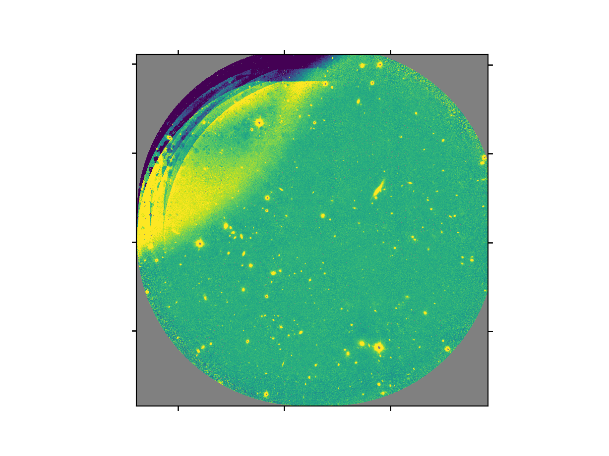
The final product file will have a _image.fits suffix and it is shown below.

The output stack units are in electrons (header keyword BUNIT=electrons). The output stack is stored in a multi-extension FITS (MEF) file. The science signal is in the “SCI” extension, the variance is in the “VAR” extension, and the data quality plane (mask) is in the “DQ” extension.

Warning

The upper-left quadrant of this science sequence is rather messy. This is caused by the PWFS2 guide probe (see Emission from PWFS2 guide probe). Photometry in this portion of the image is likely to be seriously compromised.