3. Example 1-A: Extended source - Using the “reduce” command
In this example we will reduce a NIRI observation of an extended source using the “reduce” command that is operated directly from the unix shell. Just open a terminal and load the DRAGONS conda environment to get started.
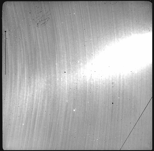
This observation is a simple dither on target, a galaxy, with offset to sky.
3.1. The dataset
If you have not already, download and unpack the tutorial’s data package. Refer to Downloading the tutorial datasets for the links and simple instructions.
The dataset specific to this example is described in:
Here is a copy of the table for quick reference.
| Science | N20160102S0270-274 (on-target)
N20160102S0275-279 (on-sky)
|
| Science darks | N20160102S0423-432 (20 sec, like Science)
|
| Flats | N20160102S0373-382 (lamps-on)
N20160102S0363-372 (lamps-off)
|
| Short darks | N20160103S0463-472
|
| Standard star | N20160102S0295-299
|
3.2. Set up the Local Calibration Manager
DRAGONS comes with a local calibration manager and a local light weight database that uses the same calibration association rules as the Gemini Observatory Archive. This allows “reduce” to make requests for matching processed calibrations when needed to reduce a dataset.
Let’s set up the local calibration manager for this session.
In ~/.geminidr/, create or edit the configuration file rsys.cfg as
follow:
[calibs]
standalone = True
database_dir = <where_the_data_package_is>/niriimg_tutorial/playground
This simply tells the system where to put the calibration database, the database that will keep track of the processed calibrations we are going to send to it.
Note
~ in the path above refers to your home directory. Also, don’t
miss the dot in .geminidr.
Then initialize the calibration database:
caldb init
That’s it. It is ready to use.
You can add processed calibrations with caldb add <filename> (we will
later), list the database content with caldb list, and
caldb remove <filename> to remove a file from the database (it will not
remove the file on disk.) (See the “caldb” documentation for more details.)
3.3. Create file lists
This data set contains science and calibration frames. For some programs, it could have different observed targets and different exposure times depending on how you like to organize your raw data.
The DRAGONS data reduction pipeline does not organize the data for you. You have to do it. DRAGONS provides tools to help you with that.
The first step is to create input file lists. The tool “dataselect” helps with that. It uses Astrodata tags and “descriptors” to select the files and send the filenames to a text file that can then be fed to “reduce”. (See the Astrodata User Manual for information about Astrodata.)
First, navigate to the playground directory in the unpacked data package.
3.3.1. Two lists for the darks
We have two sets of darks; one set for the science frames, the 20-second darks, and another for making the BPM, the 1-second darks. We will create two lists.
If you did not know the exposure times for the darks, you could have use a
combination of “dataselect” to select all the darks (tag DARK) and feed
that list to “showd” to show descriptor values, in this case
exposure_time. (See the descriptors page for a complete list.)
dataselect ../playdata/*.fits --tags DARK | showd -d exposure_time

-----------------------------------------------
filename                          exposure_time
-----------------------------------------------
../playdata/N20160102S0423.fits          20.002
../playdata/N20160102S0424.fits          20.002
../playdata/N20160102S0425.fits          20.002
../playdata/N20160102S0426.fits          20.002
../playdata/N20160102S0427.fits          20.002
../playdata/N20160102S0428.fits          20.002
../playdata/N20160102S0429.fits          20.002
../playdata/N20160102S0430.fits          20.002
../playdata/N20160102S0431.fits          20.002
../playdata/N20160102S0432.fits          20.002
../playdata/N20160103S0463.fits           1.001
../playdata/N20160103S0464.fits           1.001
../playdata/N20160103S0465.fits           1.001
../playdata/N20160103S0466.fits           1.001
../playdata/N20160103S0467.fits           1.001
../playdata/N20160103S0468.fits           1.001
../playdata/N20160103S0469.fits           1.001
../playdata/N20160103S0470.fits           1.001
../playdata/N20160103S0471.fits           1.001
../playdata/N20160103S0472.fits           1.001
As one can see above the exposure times all have a small fractional increment. This is just a floating point inaccuracy somewhere in the software that generates the raw NIRI FITS files. As far as we are concerned here in this tutorial, we are dealing with 20-second and 1-second darks. The tool “dataselect” is smart enough to match those exposure times as “close enough”. So, in our selection expression, we can use “1” and “20” and ignore the extra digits.
Note
If a perfect match to 1.001 were required, adding the option
--strict in dataselect would ensure an exact match.
Let’s create our two lists now.
dataselect ../playdata/*.fits --tags DARK --expr='exposure_time==1' -o darks1s.lis
dataselect ../playdata/*.fits --tags DARK --expr='exposure_time==20' -o darks20s.lis
3.3.2. A list for the flats
The flats are a sequence of lamp-on and lamp-off exposures. We just send all of them to one list.
dataselect ../playdata/*.fits --tags FLAT -o flats.lis
3.3.3. A list for the standard star
The standard stars at Gemini are normally taken as partner calibration.
You can see the observation_class of all the data using “showd”. Here
we will print the object name too.
showd ../playdata/*.fits -d observation_class,object

--------------------------------------------------------------
filename                          observation_class     object
--------------------------------------------------------------
../playdata/N20160102S0270.fits             science    SN2014J
...
../playdata/N20160102S0295.fits          partnerCal      FS 17
../playdata/N20160102S0296.fits          partnerCal      FS 17
../playdata/N20160102S0297.fits          partnerCal      FS 17
../playdata/N20160102S0298.fits          partnerCal      FS 17
../playdata/N20160102S0299.fits          partnerCal      FS 17
../playdata/N20160102S0363.fits              dayCal   GCALflat
...
../playdata/N20160103S0472.fits              dayCal       Dark
The list is abridged for presentation.
Our standard star is a “partnerCal” named “FS 17”. Since it is unique, we can use either criterion to get our list.
dataselect ../playdata/*.fits --expr='observation_class=="partnerCal"' -o stdstar.lis
Or
dataselect ../playdata/*.fits --expr='object=="FS 17"' -o stdstar.lis
3.3.4. A list for the science observations
The science frames are all the IMAGE non-FLAT frames that are also not
the standard. Since flats are tagged FLAT and IMAGE, we need to
exclude the FLAT tag.
This translates to the following expression:
dataselect ../playdata/*.fits --tags IMAGE --xtags FLAT --expr='object!="FS 17"' -o target.lis
One could have used the name of the science target too, like we did for selecting the standard star observation in the previous section. The example above shows how to exclude a tag if needed and was considered more educational.
3.4. Master Dark
We first create the master dark for the science target, then add it to the
calibration database. The name of the output master dark,
N20160102S0423_dark.fits, is written to the screen at the end of the
process.
reduce @darks20s.lis
caldb add N20160102S0423_dark.fits
The @ character before the name of the input file is the “at-file” syntax.
More details can be found in the "at-file" Facility documentation.
Note
The file name of the output processed dark is the file name of the first file in the list with _dark appended as a suffix. This the general naming scheme used by “reduce”.
3.5. Bad Pixel Mask
The DRAGONS Gemini data reduction package, geminidr, comes with a static
NIRI bad pixel mask (BPM) that gets automatically added to all the NIRI data
as they gets processed. The user can also create a supplemental, fresher BPM
from the flats and recent short darks. That new BPM is later fed to
“reduce” as a user BPM to be combined with the static BPM. Using both the
static and a fresh BPM from recent data lead to a better representation of the
bad pixels. It is an optional but recommended step.
The flats and the short darks are the inputs.
The flats must be passed first to the input list to ensure that the recipe
library associated with NIRI flats is selected. We will not use the default
recipe but rather the special recipe from that library called
makeProcessedBPM.
reduce @flats.lis @darks1s.lis -r makeProcessedBPM
The BPM produced is named N20160102S0373_bpm.fits.
The local calibration manager does not yet support BPMs so we cannot add it to the database. It is a future feature. Until then we have to pass it manually to “reduce” to use it, as we will show below.
3.6. Master Flat Field
A NIRI master flat is created from a series of lamp-on and lamp-off exposures. Each flavor is stacked, then the lamp-off stack is subtracted from the lamp-on stack.
We create the master flat field and add it to the calibration database as follow:
reduce @flats.lis -p addDQ:user_bpm=N20160102S0373_bpm.fits
caldb add N20160102S0373_flat.fits
Note how we pass in the BPM we created in the previous step. The addDQ
primitive, one of the primitives in the recipe, has an input parameter named
user_bpm. We assign our BPM to that input parameter.
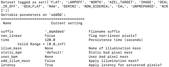
To see the list of available input parameters and their defaults, use the tool “showpars”. It needs the name of a file on which the primitive will be run because the defaults are adjusted to match the input data.
showpars ../playdata/N20160102S0363.fits addDQ
3.7. Standard Star
The standard star is reduced more or less the same way as the science target (next section) except that darks frames are not obtained for standard star observations. Therefore the dark correction needs to be turned off.
The processed flat field that we added earlier to the local calibration database will be fetched automatically. The user BPM (optional, but recommended) needs to be specified by the user.
reduce @stdstar.lis -p addDQ:user_bpm=N20160102S0373_bpm.fits darkCorrect:do_cal=skip
3.8. Science Observations
The science target is an extended source. We need to turn off the scaling of the sky because the target fills the field of view and does not represent a reasonable sky background. If scaling is not turned off in this particular case, it results in an over-subtraction of the sky frame.
The sky frame comes from off-target sky observations. We feed the pipeline all the on-target and off-target frames. The software will split the on-target and the off-target appropriately.
The master dark and the master flat will be retrieved automatically from the local calibration database. Again, the user BPM needs to be specified on the command line.
The output stack units are in electrons (header keyword BUNIT=electrons). The output stack is stored in a multi-extension FITS (MEF) file. The science signal is in the “SCI” extension, the variance is in the “VAR” extension, and the data quality plane (mask) is in the “DQ” extension.
reduce @target.lis -p addDQ:user_bpm=N20160102S0373_bpm.fits skyCorrect:scale_sky=False
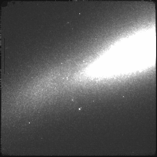
The attentive reader will note that the reduced image is slightly larger than the individual raw image. This is because of the telescope was dithered between each observation leading to a slightly larger final field of view than that of each individual image. The stacked product is not cropped to the common area, rather the image size is adjusted to include the complete area covered by the whole sequence. Of course the areas covered by less than the full stack of images will have a lower signal-to-noise. The final MEF file has three named extensions, the science (SCI), the variance (VAR), and the data quality plance (DQ).