2. Data Reduction with “reduce”

This chapter will guide you on reducing GSAOI data using command line tools. In this example we reduce a GSAOI observation of the resolved outskirt of a nearby galaxy. The observation is a dither-on-target with offset-to-sky sequence. Just open a terminal to get started.

While the example cannot possibly cover all situations, it will help you get acquainted with the reduction of GSAOI data with DRAGONS. We encourage you to look at the Tips and Tricks and Issues and Limitations chapters to learn more about GSAOI data reduction.

DRAGONS installation comes with a set of scripts that are used to reduce astronomical data. The most important script is called “reduce”, which is extensively explained in the Recipe System Users Manual. It is through that command that a DRAGONS reduction is launched.

For this tutorial, we will be also using the following supplemental tools: “dataselect”, “showd”, “typewalk”, and “caldb”.

2.1. The dataset

If you have not already, download and unpack the tutorial’s data package. Refer to Downloading the tutorial datasets for the links and simple instructions.

The dataset specific to this example is described in:

About the dataset.

Here is a copy of the table for quick reference.

Science	S20170505S0095-110	Kshort-band, on target, 60 s
Flats	S20170505S0030-044 S20170505S0060-074	Lamp on, Kshort, for science Lamp off, Kshort, for science
Standard star	S20170504S0114-117	Kshort, standard star, 30 s

Note

A master dark is not needed for GSAOI. The dark current is very low.

2.2. Set up the Local Calibration Manager

DRAGONS comes with a local calibration manager that uses the same calibration association rules as the Gemini Observatory Archive. This allows reduce to make requests to a local light-weight database for matching processed calibrations when needed to reduce a dataset.

Let’s set up the local calibration manager for this session.

In ~/.geminidr/, create or edit the configuration file rsys.cfg as follow:

[calibs]
standalone = True
database_dir = ${path_to_my_data}/gsaoiimg_tutorial/playground

This simply tells the system where to put the calibration database, the database that will keep track of the processed calibrations we are going to send to it.

Note

The tilde (~) in the path above refers to your home directory. Also, mind the dot in .geminidr.

Then initialize the calibration database:

caldb init

That’s it! It is ready to use!

You can add processed calibrations with caldb add <filename> (we will later), list the database content with caldb list, and caldb remove <filename> to remove a file only from the database (it will not remove the file on disk). For more the details, check the Recipe System Local Calibration Manager documentation, caldb.

2.3. Check files

For this example, all the raw files we need are in the same directory called ../playdata/. Let us learn a bit about the data we have.

Ensure that you are in the playground directory and that the conda environment that includes DRAGONS has been activated.

Let us call the command tool “typewalk”:

$ typewalk -d ../playdata/

directory:  /data/workspace/gsaoiimg_tutorial/playdata
     S20170504S0114.fits ............... (GEMINI) (GSAOI) (IMAGE) (RAW) (SIDEREAL) (SOUTH) (UNPREPARED)
     ...
     S20170505S0030.fits ............... (AZEL_TARGET) (CAL) (DOMEFLAT) (FLAT) (GEMINI) (GSAOI) (IMAGE) (LAMPON) (NON_SIDEREAL) (RAW) (SOUTH) (UNPREPARED)
     ...
     S20170505S0060.fits ............... (AZEL_TARGET) (CAL) (DOMEFLAT) (FLAT) (GEMINI) (GSAOI) (IMAGE) (LAMPOFF) (NON_SIDEREAL) (RAW) (SOUTH) (UNPREPARED)
     ...
     S20170505S0095.fits ............... (GEMINI) (GSAOI) (IMAGE) (RAW) (SIDEREAL) (SOUTH) (UNPREPARED)
     ...
     S20170505S0110.fits ............... (GEMINI) (GSAOI) (IMAGE) (RAW) (SIDEREAL) (SOUTH) (UNPREPARED)
Done DataSpider.typewalk(..)

This command will open every FITS file within the folder passed after the -d flag (recursively) and will print an unsorted table with the file names and the associated tags. For example, calibration files will always have the CAL tag. Flat images will always have the FLAT tag. This means that we can start getting to know a bit more about our data set just by looking at the tags. The output above was trimmed for presentation.

2.4. Create File lists

This data set contains science and calibration frames. For some program, it could have different observed targets and different exposure times depending on how you like to organize your raw data.

The DRAGONS data reduction pipeline does not organize the data for you. You have to do it. DRAGONS provides tools to help you with that.

The first step is to create lists that will be used in the data reduction process. For that, we use “dataselect”. Please, refer to the “dataselect” documentation for details regarding its usage.

2.4.1. A list for the flats

Let us create the list containing the domeflats:

$ dataselect --tags FLAT ../playdata/*.fits -o flats_Kshort.list

We know that our dataset has only one filter (Kshort). If our dataset contained data with more filters, we would have had to use the --expr option to select the appropriate filter as follow:

$ dataselect --tags FLAT --expr "filter_name=='Kshort'" ../playdata/*.fits -o flats_Kshort.list

Note

To see the name of the filter, use “showd” (show descriptor):

$ showd ../playdata/*.fits -d filter_name
----------------------------------------------------
filename                                 filter_name
----------------------------------------------------
../playdata/S20170504S0114.fits   Kshort_G1105&Clear
...
...

2.4.2. A list for the standard star

In this case we have only one standard star. Indeed, we can confirm that by selecting on partner calibrations and showing the object name:

$ dataselect --expr 'observation_class=="partnerCal"' ../playdata/*.fits | showd -d object
----------------------------------------
filename                          object
----------------------------------------
../playdata/S20170504S0114.fits     9132
../playdata/S20170504S0115.fits     9132
../playdata/S20170504S0116.fits     9132
../playdata/S20170504S0117.fits     9132

If we had more than one object, a list for each standard star is created by using the object descriptor as a selection criterium in “dataselect”:

$ dataselect --expr 'object=="9132"' ../playdata/*.fits -o std_9132.list

2.4.3. A list for the science observations

The rest is the data with your science target. Before we create a new list, let us check that indeed we have only one science target and a unique exposure time:

$ dataselect --expr 'observation_class=="science"' ../playdata/*.fits | showd -d object,exposure_time
---------------------------------------------------------
filename                           object   exposure_time
---------------------------------------------------------
../playdata/S20170505S0095.fits   NGC5128            60.0
../playdata/S20170505S0096.fits   NGC5128            60.0
...
../playdata/S20170505S0109.fits   NGC5128            60.0
../playdata/S20170505S0110.fits   NGC5128            60.0

Just to demonstrate how expression are built, let us consider that we need to select only the files for which object is NGC5128 and exposure_time is 60 seconds. We also want to pass the output to a new list:

$ dataselect --expr '(observation_class=="science" and exposure_time==60.)' ../playdata/*.fits -o science.list

2.5. Create a Master Flat Field

The GSAOI Kshort master flat is created from a series of lamp-on and lamp-off dome exposures. They should all have the same exposure time. Each flavor is stacked (averaged), then the lamp-off stack is subtracted from the lamp-on stack and the result normalized.

We create the master flat field and add it to the calibration manager as follows:

$ reduce @flats_Kshort.list
$ caldb add S20170505S0030_flat.fits

The master flat file is found in two places: inside the same folder where you ran reduce and inside the calibrations/processed_flats/ folder, for safekeeping. Here is an example of a master flat:

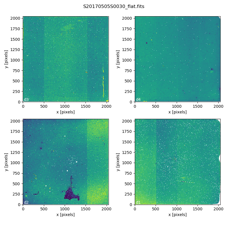
Master Flat - K-Short Band

Note that this figure shows the masked pixels in white color but not all the detector features are masked. For example, the “Christmas Tree” on detector 2 can be easily noticed but was not masked.

2.6. Reduce Standard Star

The standard star is reduced essentially the same way as the science target (next section). The processed flat field that we added earlier to the local calibration database will be fetched automatically. Also, in this case the standard star was obtained using ROIs (Regions-of-Interest) which do not match the flat field. The software will recognize that the flat field is still valid and will crop it to match the ROIs.

$ reduce @std_9132.list

To stack, the tool disco_stu is needed for GSAOI. It is discussed later in this chapter.

$ disco `dataselect *_skyCorrected.fits --expr='observation_class=="partnerCal"'`

2.7. Reduce the Science Images

This is an observation of a galaxy with offset to sky. We need to turn off the additive offsetting of the sky because the target fills the field of view and does not represent a reasonable sky background. If the offsetting is not turned off in this particular case, it results in an over-subtraction of the sky frame.

Note

Unlike the other near-IR instruments, the additive offset_sky parameter is used by default to adjust the sky frame background for GSAOI instead of the multiplicative scale_sky parameter. It was found to work better when the sky background per pixel is very low, which is common due to the short exposure time needed to avoid saturating stars and the small pixel scale. The reader is encourage to experiment with scale_sky if offset_sky does not seem to lead to an optimal sky subtraction.

(Remember that when the source is extended, both parameters normally need to be turned off.)

The sky frame comes from off-target sky observations. We feed the pipeline all the on-target and off-target frames. The software will split the on-target and the off-target appropriately using information in the headers.

Once we have our calibration files processed and added to the database, ready for retrieval, we can run reduce on our science data.

$ reduce @science.list -p skyCorrect:offset_sky=False

This command will generate flat corrected and sky subtracted files but will not stack them. You can find which file is which by its suffix (_flatCorrected or _skyCorrected). The on-target files are the ones that have been sky subtracted (_skyCorrected). There should be nine of them.

The frames are not stacked because of the high level of distortion in the GSAOI images that requires special software to correct and properly stack. The tool disco_stu (next section) must be used to stack GSAOI science data.

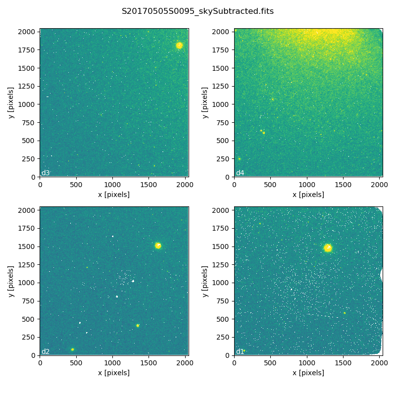
S20170505S0095 - Flat corrected and sky subtracted

The figure above shows an example of the sky-subtracted frames. The masked pixels are represented in white color.

2.8. Stack Sky-Subtracted Science Images

The final step is to stack the images. For that, you must be aware that GSAOI images are highly distorted and that this distortion must be corrected before stacking. The tool for distortion correction and image stacking is disco_stu.

Note

disco_stu is installed with conda when the standard Gemini software installation instructions are followed. To install after the fact:

conda install disco_stu

The simplest use of disco_stu is to run the command disco on the files to be stacked.

$ disco `dataselect *_skyCorrected.fits --expr 'observation_class=="science"'` -o my_Kshort_stack.fits

By default, disco will write the output file as disco_stack.fits, the -o flag allows us to override that and choose the name of the output stack.

For absolute distortion correction and astrometry, disco_stu can use a reference catalog provided by the user. Without a reference catalog, like above, only the relative distortion between the frames is accounted for. For more information about disco_stu see the disco_stu.pdf manual in $CONDA_PREFIX/share/disco_stu.

The output stack units are in electrons (header keyword BUNIT=electrons). The output stack is stored in a multi-extension FITS (MEF) file. The science signal is in the “SCI” extension, the variance is in the “VAR” extension, and the data quality plane (mask) is in the “DQ” extension.

The final image is shown below.

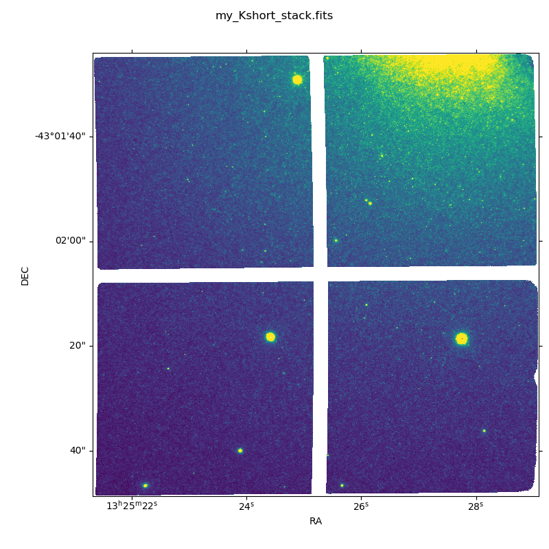
Sky Subtracted and Stacked Final Image