Example 1-B: Point source through keyhole - Using the “Reduce” class

A reduction can be initiated from the command line as shown in Example 1-A: Point source through keyhole - Using the “reduce” command and it can also be done programmatically as we will show here. The classes and modules of the RecipeSystem can be accessed directly for those who want to write Python programs to drive their reduction. In this example we replicate the command line reduction from Example 1-A, this time using the Python interface instead of the command line. Of course what is shown here could be packaged in modules for greater automation.

The dataset

If you have not already, download and unpack the tutorial’s data package. Refer to Downloading the tutorial datasets for the links and simple instructions.

The dataset specific to this example is described in:

Dataset for example 1: Point source through the acquisition keyhole.

Here is a copy of the table for quick reference.

Science	N20120117S0014-33 (J-band, on-target)
Science darks	N20120102S0538-547 (60 sec, like Science)
Flats	N20120117S0034-41 (lamps-on) N20120117S0042-49 (lamps-off)

Setting up

First, navigate to the playground directory in the unpacked data package.

The first steps are to import libraries, set up the calibration manager, and set the logger.

Importing Libraries

import glob

# DRAGONS imports
from recipe_system.reduction.coreReduce import Reduce
from recipe_system import cal_service
from gempy.adlibrary import dataselect

The dataselect module will be used to create file lists for the darks, the flats and the science observations. The cal_service package is our interface to the local calibration database. Finally, the Reduce class is used to set up and run the data reduction.

Setting up the logger

We recommend using the DRAGONS logger. (See also Double messaging issue.)

from gempy.utils import logutils
logutils.config(file_name='gnirs_tutorial.log')

Set up the Local Calibration Manager

DRAGONS comes with a local calibration manager and a local light weight database that uses the same calibration association rules as the Gemini Observatory Archive. This allows the Reduce instance to make requests for matching processed calibrations when needed to reduce a dataset.

Let’s set up the local calibration manager for this session.

In ~/.geminidr/, edit the configuration file rsys.cfg as follow:

[calibs]
standalone = True
database_dir = <where_the_data_package_is>/gnirsimg_tutorial/playground

This tells the system where to put the calibration database, the database that will keep track of the processed calibration we are going to send to it.

Note

The tilde (~) in the path above refers to your home directory. Also, mind the dot in .geminidr.

The calibration database is initialized and the calibration service is configured like this:

caldb = cal_service.CalibrationService()
caldb.config()
caldb.init()

cal_service.set_calservice()

The calibration service is now ready to use. If you need more details, check the “caldb” documentation in the Recipe System User Manual.

Create file lists

The next step is to create input file lists. The tool dataselect helps with that. It uses Astrodata tags and descriptors to select the files and store the filenames to a Python list that can then be fed to the Reduce class. (See the Astrodata User Manual for information about Astrodata and for a list of descriptors.)

The first list we create is a list of all the files in the playdata directory.

all_files = glob.glob('../playdata/*.fits')
all_files.sort()

We will search that list for files with specific characteristics. We use the all_files list as an input to the function dataselect.select_data() . The function’s signature is:

select_data(inputs, tags=[], xtags=[], expression='True')

We show several usage examples below.

A list for the darks

There is only one set of 60-second darks in the data package. To create the list, one simply need to select on the DARK tag:

darks60 = dataselect.select_data(all_files, ['DARK'])

If there was a need to select specifically on the 60-second darks, the command would use the exposure_time descriptor:

darks60 = dataselect.select_data(
    all_files,
    ['DARK'],
    [],
    dataselect.expr_parser('exposure_time==60')
)

Note

All expressions need to be processed with dataselect.expr_parser.

A list for the flats

The flats are a sequence of lamp-on and lamp-off exposures. We just send all of them to one list.

flats = dataselect.select_data(all_files, ['FLAT'])

A list for the science observations

The science frames are all the IMAGE non-FLAT frames in the data package. They are also the J filter images that are non-FLAT. And they are the ones with an object name GRB120116A. Those are all valid ways to select the science observations. Here we show all three ways as examples; of course, just one is required.

target = dataselect.select_data(all_files, ['IMAGE'], ['FLAT'])

# Or...
target = dataselect.select_data(
    all_files,
    [],
    ['FLAT'],
    dataselect.expr_parser('filter_name=="J"')
)

# Or...
target = dataselect.select_data(
    all_files,
    [],
    [],
    dataselect.expr_parser('object=="GRB120116A"')
)

Pick the one you prefer, in this case, they all yield the same list.

Master Dark

We first create the master dark for the science target, then add it to the calibration database. The name of the output master dark is N20120102S0538_dark.fits. The output is written to disk and its name is stored in the Reduce instance. The calibration service expects the name of a file on disk.

reduce_darks = Reduce()
reduce_darks.files.extend(darks60)
reduce_darks.runr()

caldb.add_cal(reduce_darks.output_filenames[0])

The Reduce class is our reduction “controller”. This is where we collect all the information necessary for the reduction. In this case, the only information necessary is the list of input files which we add to the files attribute. The Reduce.runr{} method is where the recipe search is triggered and where it is executed.

Note

The file name of the output processed dark is the file name of the first file in the list with _dark appended as a suffix. This the general naming scheme used by the Recipe System.

Master Flat Field

A GNIRS master flat is created from a series of lamp-on and lamp-off exposures. Each flavor is stacked, then the lamp-off stack is subtracted from the lamp-on stack.

We create the master flat field and add it to the calibration database as follows:

reduce_flats = Reduce()
reduce_flats.files.extend(flats)
reduce_flats.runr()

caldb.add_cal(reduce_flats.output_filenames[0])

Science Observations

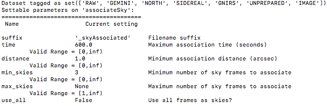
The science target is a point source. The sequence dithers on-target, moving the source across the thin keyhole aperture. The sky frames for each science image will be the adjacent dithered frames obtained within a certain time limit. The default for GNIRS keyhole images is “within 600 seconds”. This can be seen by using the “showpars” command-line tool:

showpars ../playdata/N20120117S0014.fits associateSky

Both the master dark and the master flat are in our local calibration database. For any other Gemini facility instrument, they would both be retrieved automatically by the calibration manager. However, GNIRS not being an imager, and the keyhole being normally used only for acquisition, it turns out that there are no calibration association rules between GNIRS keyhole images and darks. This is a recently discovered limitation that we plan to fix in a future release. In the meantime, we are not stuck, we can simply specify the dark on the command line. The flat will be retrieved automatically.

from recipe_system.utils.reduce_utils import normalize_ucals
mycalibrations = ['processed_dark:N20120102S0538_dark.fits']

reduce_target = Reduce()
reduce_target.files.extend(target)
ucals_dict = normalize_ucals(reduce_target.files, mycalibrations)
reduce_target.ucals = ucals_dict
reduce_target.runr()

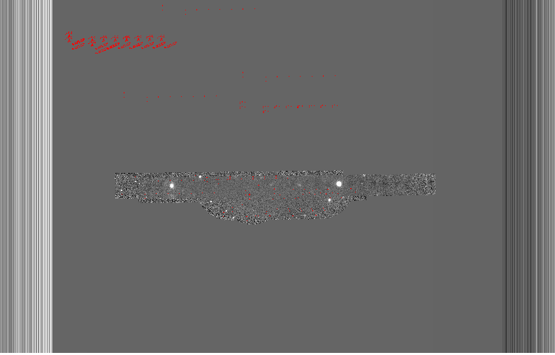
The output stack units are in electrons (header keyword BUNIT=electrons). The output stack is stored in a multi-extension FITS (MEF) file. The science signal is in the “SCI” extension, the variance is in the “VAR” extension, and the data quality plane (mask) is in the “DQ” extension.

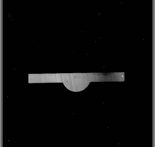
Below are a raw image (top) and the final stacked image (bottom). The stack keeps all the pixels and is never cropped to only the common area. Of course the areas covered by less than the full stack of images will have a lower signal-to-noise.