Example 1 - Keyhole imaging of two stars with dithers - Using the “reduce” command line

In this example we will reduce a GNIRS keyhole imaging observation of a point source using the “reduce” command that is operated directly from the unix shell. Just open a terminal to get started.

This observation is a simple dither on target.

The dataset

If you have not already, download and unpack the tutorial’s data package. Refer to the Downloading the tutorial datasets for the links and simple instructions.

The dataset specific to this example is described in:

Example 1 - Datasets descriptions.

Here is a copy of the table for quick reference.

Science	N20120117S0014-33 (J-band, on-target)
Science darks	N20120102S0538-547 (60 sec, like Science)
Flats	N20120117S0034-41 (lamps-on) N20120117S0042-49 (lamps-off)
BPM	bpm_20100716_gnirs_gnirsn_11_full_1amp.fits

Set up the Local Calibration Manager

Important

Remember to set up the calibration service.

Instructions to configure and use the calibration service are found in Setting up the Calibration Service, specifically the these sections: The Configuration File and Usage from the Command Line.

Create file lists

This data set contains science and calibration frames. For some programs, it could have different observed targets and different exposure times depending on how you like to organize your raw data.

The DRAGONS data reduction pipeline does not organize the data for you. You have to do it. DRAGONS provides tools to help you with that.

The first step is to create input file lists. The tool “dataselect” helps with that. It uses Astrodata tags and “descriptors” to select the files and send the filenames to a text file that can then be fed to “reduce”. (See the Astrodata User Manual for information about Astrodata.)

First, navigate to the playground directory in the unpacked data package.

cd <path>/gnirsim_tutorial/playground

A list of the darks

There is only one set of 60-second darks in the data package. To create the list, one simply needs to select on the DARK tag:

dataselect ../playdata/example1/*.fits --tags DARK -o darks60.lis

If there was a need to select specifically on the 60-second darks, the command would use the exposure_time descriptor:

dataselect ../playdata/example1/*.fits --tags DARK --expr='exposure_time==60' -o darks60.lis

A list for the flats

The flats are a sequence of lamp-on and lamp-off exposures. We just send all of them to one list.

dataselect ../playdata/example1/*.fits --tags FLAT -o flats.lis

A list for the science observations

The science frames are all the IMAGE non-FLAT frames in the data package. They are also the J filter images that are non-FLAT. And they are the ones with an object name GRB120116A. Those are all valid ways to select the science observations. Here we show all three ways as examples; of course, just one is required.

dataselect ../playdata/example1/*.fits --tags IMAGE --xtags FLAT -o target.lis

dataselect ../playdata/example1/*.fits --xtags FLAT --expr='filter_name=="J"' -o target.lis

dataselect ../playdata/example1/*.fits --expr='object=="GRB120116A"' -o target.lis

Pick the one you prefer, they all yield the same list.

Note

For GNIRS data, it is useful to check the World Coordinate System (WCS) of the science data.

$ reduce -r checkWCS @target.lis

Please see details in Checking WCS of science frames in the Tips and Tricks chapter.

Master Dark

We first create the master dark for the science target, then add it to the calibration database. The name of the output master dark, N20120102S0538_dark.fits, is written to the screen at the end of the process.

reduce @darks60.lis

The @ character before the name of the input file is the “at-file” syntax. More details can be found in the "at-file" Facility documentation.

Because the database was given the “store” option in the dragonsrc file, the processed dark will be automatically added to the database at the end of the recipe.

Note

The file name of the output processed dark is the file name of the first file in the list with _dark appended as a suffix. This is the general naming scheme used by “reduce”.

Note

If you wish to inspect the processed calibrations before adding them to the calibration database, remove the “store” option attached to the database in the dragonsrc configuration file. You will then have to add the calibrations manually following your inspection, eg.

caldb add N20120102S0538_dark.fits

Bad Pixel Mask

Starting with DRAGONS v3.1, the bad pixel masks (BPMs) are now handled as calibrations. They are downloadable from the archive instead of being packaged with the software. They are automatically associated like any other calibrations. This means that the user now must download the BPMs along with the other calibrations and add the BPMs to the local calibration manager.

See Getting Bad Pixel Masks from the archive in Tips and Tricks to learn about the various ways to get the BPMs from the archive.

To add the static BPM included in the data package to the local calibration database:

caldb add ../playdata/example1/bpm*.fits

Master Flat Field

A GNIRS master flat is created from a series of lamp-on and lamp-off exposures. Each flavor is stacked, then the lamp-off stack is subtracted from the lamp-on stack.

We create the master flat field and add it to the calibration database as follows:

reduce @flats.lis

Science Observations

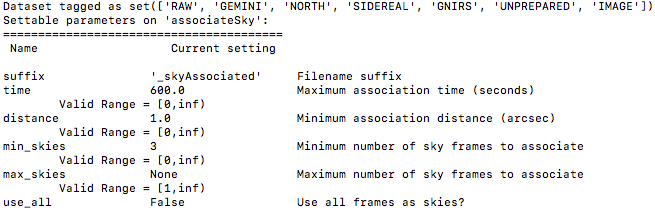
The science targets are two point sources. The sequence dithers on-target, moving the sources across the thin keyhole aperture. The sky frames for each science image will be the adjacent dithered frames obtained within a certain time limit. The default for GNIRS keyhole images is “within 600 seconds”. This can be seen by using “showpars”:

showpars ../playdata/example1/N20120117S0014.fits associateSky

The BPM, the master dark and the master flat are in our local calibration database. For any other Gemini facility instrument, they would both be retrieved automatically by the calibration manager. However, GNIRS not being an imager, and the keyhole being normally used only for acquisition, it turns out that there are no calibration association rules between GNIRS keyhole images and darks. We can specify the dark on the command line. The flat will be retrieved automatically.

reduce @target.lis --user_cal processed_dark:N20120102S0538_dark.fits

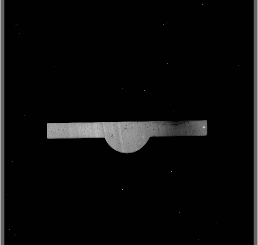
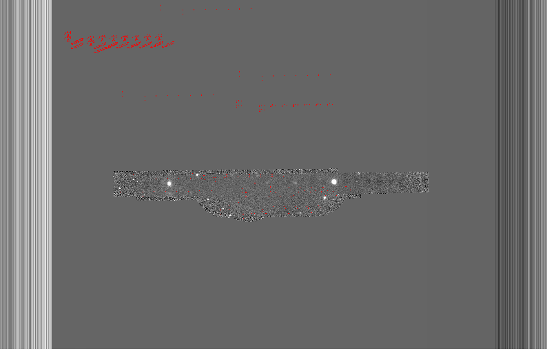
The output stack units are in electrons (header keyword BUNIT=electrons). The output stack is stored in a multi-extension FITS (MEF) file. The science signal is in the “SCI” extension, the variance is in the “VAR” extension, and the data quality plane (mask) is in the “DQ” extension.

Below are a raw image (top) and the final stacked image (bottom). The stack keeps all the pixels and is never cropped to only the common area. Of course the areas covered by less than the full stack of images will have a lower signal-to-noise.