4.3. Example 1 - Standard Resolution One Target - Using the “Reduce” API

In this example we will reduce a GHOST observation of the star XX Oph using the Reduce class that serves as the main API to the DRAGONS pipeline.

This observation uses IFU-1 for the target. IFU-2 is stowed.

4.3.1. The dataset

If you have not already, download and unpack the tutorial’s data package. Refer to Downloading tutorial datasets for the links and simple instructions.

The dataset specific to this example is described in:

Example 1 - Datasets descriptions.

Here is a copy of the table for quick reference.

Science	S20230416S0079 (blue:2x2,slow; red:2x2,medium)
Science biases	S20230417S0011-015
Science Flats	S20230416S0047 (1x1; blue:slow; red:medium)
Science Arcs	S20230416S0049-51 (1x1)
Flats Biases	S20230417S0036-40 (1x1; blue:slow; red:medium)
Arc Biases	S20230417S0036-40 (1x1; blue:slow; red:medium)
Standard (CD -32 9927)	S20230416S0073 (blue:2x2,slow; red:2x2,medium)
Standard biases	In this case, the calibrations for the science can be used for the standard star.
Standard flats
Standard arc
Std flat biases
Std arc biases
BPMs	bpm_20220601_ghost_blue_11_full_4amp.fits bpm_20220601_ghost_red_11_full_4amp.fits From archive, not data package.
BPMs

4.3.2. Setting up

Before you launch Python, navigate to your work directory in the unpacked data package.

cd <path>/gmosls_tutorial/playground

The first steps are to import libraries, set up the calibration manager, and set the logger.

4.3.2.1. Importing libraries

import glob
import os

import astrodata
import gemini_instruments
from recipe_system.reduction.coreReduce import Reduce
from gempy.adlibrary import dataselect

The dataselect module will be used to create file lists for the biases, the flats, the arcs, the standard, and the science observations. The Reduce class is used to set up and run the data reduction.

4.3.2.2. Setting up the logger

We recommend using the DRAGONS logger. (See also Double messaging issue.)

from gempy.utils import logutils
logutils.config(file_name='ghost_tutorial.log')

4.3.2.3. Set up the Calibration Service

Important

Remember to set up the calibration service.

Instructions to configure and use the calibration service are found in Setting up the Calibration Service, specifically the these sections: The Configuration File and Usage from the API.

4.3.3. The Files

Unlike for other Gemini instruments, the GHOST raw data are “bundles”. They contain multiple exposures from the red channel, multiple exposures for the blue channel, and multiple slit-viewer images.

To keep our work directory clean, at least while learning how to reduce GHOST data, we will de-bundle the files we need as we need them and create list of data to reduce as we need them.

It might be tempting to de-bundle all the data at once, but beware of memory issues. GHOST raw bundles are very large. You will also be drowned in files.

Let’s inspect the data. (It take a little long to run, the bundle files are large.) From a terminal:

cd <path>/ghost_tutorial/playground
showd ../playdata/example1/*.fits -d object,detector_x_bin,detector_y_bin,read_mode

---------------------------------------------------------------------------------------------------------------------------------------------------------------------------------------
filename                                        object                      detector_x_bin                      detector_y_bin                                                read_mode
---------------------------------------------------------------------------------------------------------------------------------------------------------------------------------------
../playdata/example1/S20230416S0047.fits                            GCALflat   {'blue': 1, 'red': 1, 'slitv': 2}   {'blue': 1, 'red': 1, 'slitv': 2}   {'blue': 'slow', 'red': 'medium', 'slitv': 'standard'}
../playdata/example1/S20230416S0049.fits                                ThAr   {'blue': 1, 'red': 1, 'slitv': 2}   {'blue': 1, 'red': 1, 'slitv': 2}   {'blue': 'slow', 'red': 'medium', 'slitv': 'standard'}
../playdata/example1/S20230416S0050.fits                                ThAr   {'blue': 1, 'red': 1, 'slitv': 2}   {'blue': 1, 'red': 1, 'slitv': 2}   {'blue': 'slow', 'red': 'medium', 'slitv': 'standard'}
../playdata/example1/S20230416S0051.fits                                ThAr   {'blue': 1, 'red': 1, 'slitv': 2}   {'blue': 1, 'red': 1, 'slitv': 2}   {'blue': 'slow', 'red': 'medium', 'slitv': 'standard'}
../playdata/example1/S20230416S0073.fits                         CD -32 9927   {'blue': 2, 'red': 2, 'slitv': 2}   {'blue': 2, 'red': 2, 'slitv': 2}   {'blue': 'slow', 'red': 'medium', 'slitv': 'standard'}
../playdata/example1/S20230416S0079.fits                              XX Oph   {'blue': 2, 'red': 2, 'slitv': 2}   {'blue': 2, 'red': 2, 'slitv': 2}   {'blue': 'slow', 'red': 'medium', 'slitv': 'standard'}
../playdata/example1/S20230417S0011.fits                                Bias   {'blue': 2, 'red': 2, 'slitv': 2}   {'blue': 2, 'red': 2, 'slitv': 2}   {'blue': 'slow', 'red': 'medium', 'slitv': 'standard'}
../playdata/example1/S20230417S0012.fits                                Bias   {'blue': 2, 'red': 2, 'slitv': 2}   {'blue': 2, 'red': 2, 'slitv': 2}   {'blue': 'slow', 'red': 'medium', 'slitv': 'standard'}
../playdata/example1/S20230417S0013.fits                                Bias   {'blue': 2, 'red': 2, 'slitv': 2}   {'blue': 2, 'red': 2, 'slitv': 2}   {'blue': 'slow', 'red': 'medium', 'slitv': 'standard'}
../playdata/example1/S20230417S0014.fits                                Bias   {'blue': 2, 'red': 2, 'slitv': 2}   {'blue': 2, 'red': 2, 'slitv': 2}   {'blue': 'slow', 'red': 'medium', 'slitv': 'standard'}
../playdata/example1/S20230417S0015.fits                                Bias   {'blue': 2, 'red': 2, 'slitv': 2}   {'blue': 2, 'red': 2, 'slitv': 2}   {'blue': 'slow', 'red': 'medium', 'slitv': 'standard'}
../playdata/example1/S20230417S0036.fits                                Bias   {'blue': 1, 'red': 1, 'slitv': 2}   {'blue': 1, 'red': 1, 'slitv': 2}   {'blue': 'slow', 'red': 'medium', 'slitv': 'standard'}
../playdata/example1/S20230417S0037.fits                                Bias   {'blue': 1, 'red': 1, 'slitv': 2}   {'blue': 1, 'red': 1, 'slitv': 2}   {'blue': 'slow', 'red': 'medium', 'slitv': 'standard'}
../playdata/example1/S20230417S0038.fits                                Bias   {'blue': 1, 'red': 1, 'slitv': 2}   {'blue': 1, 'red': 1, 'slitv': 2}   {'blue': 'slow', 'red': 'medium', 'slitv': 'standard'}
../playdata/example1/S20230417S0039.fits                                Bias   {'blue': 1, 'red': 1, 'slitv': 2}   {'blue': 1, 'red': 1, 'slitv': 2}   {'blue': 'slow', 'red': 'medium', 'slitv': 'standard'}
../playdata/example1/S20230417S0040.fits                                Bias   {'blue': 1, 'red': 1, 'slitv': 2}   {'blue': 1, 'red': 1, 'slitv': 2}   {'blue': 'slow', 'red': 'medium', 'slitv': 'standard'}

4.3.4. Bad Pixel Mask

Starting with DRAGONS v3.1, the bad pixel masks (BPMs) are handled as calibrations. They are downloadable from the archive instead of being packaged with the software. They are automatically associated like any other calibrations. This means that the user can now download the BPMs along with the other calibrations and add the BPMs to the local calibration manager.

For this tutorial, the BPMs are not included in the data package. See Downloading tutorial datasets for a link to download them.

Once you have them locally, add them to the calibration database.

bpms = glob.glob('../playdata/example1/bpm*')
for bpm in bpms:
    caldb.add_cal(bpm)

4.3.5. Create the list of bundles

The next step is to create input file lists. The module dataselect helps with that. It uses Astrodata tags and descriptors to select the files and store the filenames to a Python list that can then be fed to the Reduce class. (See the Astrodata User Manual for information about Astrodata and for a list of descriptors.)

The first list we create is a list of all the bundles in the playdata directory.

all_bundles = glob.glob('../playdata/example1/*.fits')
all_bundles.sort()

We will search that list for files with specific characteristics. We use the all_bundles list as an input to the function dataselect.select_data() . The function’s signature is:

select_data(inputs, tags=[], xtags=[], expression='True')

We show several usage examples below.

4.3.6. Master Biases

In this section, we will create all the master biases that we need. Here is the list of biases we need to produce:

A bias for slit-viewer camera
A bias for science and standard, red channel
A bias for science and standard, blue channel
A bias for flat and arc, red channel
A bias for flat and arc, blue channel

The biases must match the binning and read-mode of the data they will be used on. The binning of the flats and arcs is always 1x1. While the read-mode for the flats must match the science, there is no such requirement for the arcs. If the arcs have a different read-mode from the science and flats, you will need an extra set of biases for the arc. Fortunately, this is not needed here since all the data was obtained with the same read-mode for all red and all blue exposures.

4.3.6.1. Debundle the biases

Debundle the biases and get a list of all the debundled files in the current directory.

bias_bundles = dataselect.select_data(all_bundles, ['BIAS'])

debundle_biases = Reduce()
debundle_biases.files.extend(bias_bundles)
debundle_biases.runr()

all_inputfiles = glob.glob('*.fits')
all_inputfiles.sort()

4.3.6.2. Reduce the slit biases

All the slit biases, regardless of binning or read mode in the blue and red channels, are identical. Then can all be stacked together to reduce noise.

slit_biases = dataselect.select_data(all_inputfiles, ['BIAS','SLIT'])

reduce_slit_biases = Reduce()
reduce_slit_biases.files.extend(slit_biases)
reduce_slit_biases.runr()

4.3.6.3. Reduce the science biases

redsci_biases = dataselect.select_data(
    all_inputfiles,
    ['BIAS','RED'],
    [],
    dataselect.expr_parser("binning=='2x2'")
)
bluesci_biases = dataselect.select_data(
    all_inputfiles,
    ['BIAS','BLUE'],
    [],
    dataselect.expr_parser("binning=='2x2'")
)

reduce_redsci_biases = Reduce()
reduce_redsci_biases.files.extend(redsci_biases)
reduce_redsci_biases.runr()

reduce_bluesci_biases = Reduce()
reduce_bluesci_biases.files.extend(bluesci_biases)
reduce_bluesci_biases.runr()

All the data was obtained with the same read modes. If this is not the case for your data and you need to select on read mode, use an expression like this one:

dataselect.expr_parser("binning=='2x2' and read_mode=='slow'")

Note

You may see the following error message:

ERROR - ValueError: zero-size array to reduction operation minimum which has no identity

If so, your bias frame is corrupted (all pixels have the same value) and you should find an alternative bias with the same binning and read speeds in the archive and use that instead.

4.3.6.4. Reduce the flat/arc biases

The flats and the arcs were taken in the same read mode. Therefore, we can use the same set of biases for the flats and the arcs. If they had been observed in different read modes, you would need a set for the flats and a set for the arcs. Fortunately, not the case here, one set for both.

redflatarc_biases = dataselect.select_data(
    all_inputfiles,
    ['BIAS','RED'],
    [],
    dataselect.expr_parser("binning=='1x1'")
)
blueflatarc_biases = dataselect.select_data(
    all_inputfiles,
    ['BIAS','BLUE'],
    [],
    dataselect.expr_parser("binning=='1x1'")
)

reduce_redflatarc_biases = Reduce()
reduce_redflatarc_biases.files.extend(redflatarc_biases)
reduce_redflatarc_biases.runr()

reduce_blueflatarc_biases = Reduce()
reduce_blueflatarc_biases.files.extend(blueflatarc_biases)
reduce_blueflatarc_biases.runr()

4.3.6.5. Master biases to Calibration Database

The output master biases, like all Reduce products, are written to disk in the work directory, ie. where Reduce was called. For calibrations, the final calibration files are also written in the calibrations directory, in a subdirectory representing the type of calibrations. For the biases, calibrations/processed_bias/.

This is a safe copy of the calibrations that will be needed later allowing us the freedom to clean the work directory between steps, which is particularly helpful in the case of GHOST. Because the database was given the “store” option in the dragonsrc file, the processed biases will be automatically added to the database at the end of the recipe and no additional commands are required.

Note

If you wish to inspect the processed calibrations before adding them to the calibration database, remove the “store” option attached to the database in the dragonsrc configuration file. You will then have to add the calibrations manually following your inspection, eg.

caldb add calibrations/processed_bias/*.fits

4.3.6.6. Clean up

GHOST reduction creates a lot of, often big, files in the work directory. It is recommended to clean up between each reduction phase. If you want to save the intermediate files, move them (mv) somewhere else at least. In this tutorial, we will simply delete them.

for f in glob.glob('*.fits'):
    os.remove(f)

4.3.7. Master Flats and Slit-flats

4.3.7.1. Debundle Flats

Debundle the flats and get a list of all the debundled files in the current directory.

flat_bundles = dataselect.select_data(all_bundles, ['FLAT'])

debundle_flats = Reduce()
debundle_flats.files.extend(flat_bundles)
debundle_flats.runr()

all_inputfiles = glob.glob('*.fits')
all_inputfiles.sort()

4.3.7.2. Reduce the Slit-flat

The slit-flat is required to reduce the red and blue channel flats, so it is important to reduce it first. Again, you will need to manually add it to the calibration database if your dragonsrc file is not set up to auto-store the calibrations as they are created.

slit_flats = dataselect.select_data(all_inputfiles, ['SLITFLAT'])

reduce_slit_flats = Reduce()
reduce_slit_flats.files.extend(slit_flats)
reduce_slit_flats.runr()

Note

You will see this message in the logs:

ERROR - Inputs have different numbers of SCI extensions.

You can safely ignore it. It is expected and the wording is misleading. This is not a real error.

4.3.7.3. Reduce the Flats

The flats have a 1x1 binning and must match the read mode of the science data. If the science data are binned, the software will bin the 1x1 flats to match. Reducing the flats takes a little time because of the step to trace each of the echelle orders.

red_flats = dataselect.select_data(all_inputfiles, ['FLAT','RED'])
blue_flats = dataselect.select_data(all_inputfiles, ['FLAT','BLUE'])

reduce_red_flats = Reduce()
reduce_red_flats.files.extend(red_flats)
reduce_red_flats.runr()

reduce_blue_flats = Reduce()
reduce_blue_flats.files.extend(blue_flats)
reduce_blue_flats.runr()

Note

If you are reducing out-of-focus data from the December 2023 FT run, you should add this parameter settin before you launch .run() on the red and blue flats:

reduce_xxx_flags.uparms = dict([('smoothing', 6)])

The value of 6 (the FWHM in pixels of the Gaussian smoothing kernel) applied to the slit-viewer camera images (which are in focus) seems to work well but may not be optimal. The value is stored in the header of the processed flat so it is applied automatically to the reduction of the arc and on-sky frames that use the flat. You are welcome to try other values.

4.3.7.4. Clean up

With the calibrations safely in the calibrations directory, we can clean the work directory.

for f in glob.glob('*.fits'):
    os.remove(f)

4.3.8. Arcs

The arcs have a 1x1 binning, the read mode does not matter. It does save processing if they are of the same read mode as the flats as otherwise they will need their own flats with a matching read mode as well as their own biases. If the science data are binned, the software will bin the 1x1 arcs to match.

A minimum of three arc exposures are required in each arm to eliminate cosmic rays (which can look very similar to arc lines). At the time these data were taken,each arc bundle only contained a single exposure in each of the red and blue arms, so three separate files are needed. Now each GHOST arc observation (and hence each raw bundle) contains three exposures in each arm so only one file should be needed.

4.3.8.1. Debundle the Arcs

Debundle the arcs and get a list of all the debundled files in the current directory.

arc_bundles = dataselect.select_data(all_bundles, ['ARC'])

debundle_arcs = Reduce()
debundle_arcs.files.extend(arc_bundles)
debundle_arcs.runr()

all_inputfiles = glob.glob('*.fits')
all_inputfiles.sort()

4.3.8.2. Reduce the slit-viewer data

We have 3 slit images for the arc because there are 3 arc bundles but we really just need one because the illumination of the slit by the arc lamp is stable. We grab the first one.

slit_arcs = dataselect.select_data(all_inputfiles, ['ARC','SLIT'])

reduce_slit_arcs = Reduce()
reduce_slit_arcs.files.extend(slit_arcs[0:1])
reduce_slit_arcs.runr()

4.3.8.3. Reduce the arcs

red_arcs = dataselect.select_data(all_inputfiles, ['ARC','RED'])
blue_arcs = dataselect.select_data(all_inputfiles, ['ARC','BLUE'])

reduce_red_arcs = Reduce()
reduce_red_arcs.files.extend(red_arcs[0:1])
reduce_red_arcs.runr()

reduce_blue_arcs = Reduce()
reduce_blue_arcs.files.extend(blue_arcs[0:1])
reduce_blue_arcs.runr()

Note

If you want to save a plot of the wavelength fits, add

reduce_xxx_arcs.uparms = dict([('determineWavelengthSolution:plot1d', True)])

to the Reduce instance. A PDF will be created.

4.3.8.4. Clean up

With the calibrations safely in the calibrations directory, we can clean the work directory.

for f in glob.glob('*.fits'):
    os.remove(f)

4.3.9. Spectrophotometric Standard

Unlike for GMOS, the standards are not automatically recognized as such. This is something that has not been implemented at this time. Therefore to select them, we will need to use the object’s name.

4.3.9.1. Debundle the Standard

Debundle the standard star and get a list of all the debundled files in the current directory.

std_bundles = dataselect.select_data(all_bundles,
        [],
        [],
        dataselect.expr_parser("object=='CD -32 9927'")
)

debundle_std = Reduce()
debundle_std.files.extend(std_bundles)
debundle_std.runr()

all_inputfiles = glob.glob('*.fits')
all_inputfiles.sort()

4.3.9.2. Reduce the slit-viewer data

Since we have cleaned up all the intermediate files as we went along, we are able to just select on the tag SLIT. If we had not cleaned up, we would need to use the object name like we did above.

slit_std = dataselect.select_data(all_inputfiles, ['SLIT'])

reduce_slit_std = Reduce()
reduce_slit_std.files.extend(slit_std)
reduce_slit_std.runr()

Note that four separate files are produced by this reduction and stored in the database. This is because the bundle contains four separate exposures in the red and blue spectrographs that cover different periods of time, and each needs its own slit-viewer image produced from the slit-viewer camera data taken at the same time. In general, as many calibration files will be produced as there are spectrograph exposures, unless the red and blue exposure times are the same, in which case the first exposures in each cover exactly the same period of time and so a single reduced slit-viewer image can be used for both.

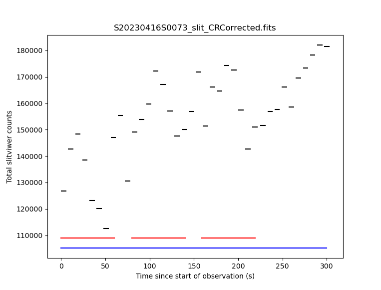
During the reduction of on-sky slit-viewer images, a plot is produced of the total flux (summed from both the red and blue slit images) as a function of time, with the durations of each of the spectrograph exposures also plotted. By default, this is written to the working directory as a PDF file with a like S20230416S0073_slit_slitflux.pdf. You can change the format with the reduce_slit_std.uparms = dict([('plotSlitFlux:format', 'png')]) or reduce_slit_std.uparms = dict([('plotSlitFlux:format', 'screen')]) where the latter option will display a plot on the screen without saving it to disk. A scatter of ~10% appears to be fairly typical, and the lower count rate in the early exposures can be traced to poorer seeing conditions, which are reported during the reduction of the spectrograph images.

4.3.9.3. Reduce the standard star

Since we have cleaned up all the intermediate files as we went along, we are able to just select on the tag RED and BLUE. If we had not cleaned up, we would need to use the object name like we did above for the bundle.

This step takes a while, with the extraction of each spectrum needing about 3 minutes. As each image is processed, the estimated seeing is reported, together with the fraction of light collected by the IFU. Here the seeing improves significantly from the first to the second red exposure, which explains the increase in the counts from the slit-viewer camera seen in the previous plot.

The spectrophotometric standard used in this tutorial is in the Gemini list and so the file containging the table of spectrophotometric data will be found automatically. If you were to use a spectrophotometric standard not on the Gemini list, you would need to provide that flux standard file with the reduce_xxx_flags.uparms = dict([('calculateSensitivity:filename', 'path/name_of_file')]). The accepted format are the “IRAF format” and any FITS table which properly describes its columns (files in the HST calspec and ESO X-Shooter libraries fulfill this criterion).

red_std = dataselect.select_data(all_inputfiles, ['RED'])
blue_std = dataselect.select_data(all_inputfiles, ['BLUE'])

reduce_red_std = Reduce()
reduce_red_std.files.extend(red_std)
reduce_red_std.recipename = 'reduceStandard'
reduce_red_std.uparms = dict([('scaleCountsToReference:tolerance', 1)])
reduce_red_std.runr()

reduce_blue_std = Reduce()
reduce_blue_std.files.extend(blue_std)
reduce_blue_std.recipename = 'reduceStandard'
reduce_blue_std.uparms = dict([('scaleCountsToReference:tolerance', 1)])
reduce_blue_std.runr()

The reduced spectrophotometric standard observations are the _standard files.

The _arraysTiled files are the last 2D images of the spectra before they gets extracted to 1D. They are saved just in case you want to inspect them. They are not used for further reduction.

For the wavelength calibration, the pipeline will try to find an arc taken before the observation and one taken after. If it finds two, it will use them both and interpolate between them to obtain a wavelength solution, but one is enough provided it is taken close enough in time (the stability of the instrument has not yet been sufficiently well quantified to say what “close enough” means, but here the arcs are taken on the same night so that is definitely OK). This is what happens here: the software finds a “before” arc, but no “after” arc. So, do not be alarmed by the messages saying that it failed to find an arc, it’s okay, it got one, it’s enough.

This standard observation has three red arm exposures whose counts can be scaled to match the level of the first frame and then stacked. By default, the scaleCountsToReference primitive only scales by the exposure time (which is the same for all these exposures), so no scaling will occur. This choice of default is to prevent erroneous scaling factors being calculated when the signal-to-noise ratio in the data are low, but that is not the case here so we can trust the ratios calculated by the software. Setting a tolerance of 1 indicates that the calculated ratios should be used whatever they are, whereas a value of, for example, 0.1 means that the ratio should only be used if it is within 10% of that expected from the relative exposure times. If the calculated ratio is outside this range, then the relative exposure times will be used to scale the data. In this case the second and third exposures are brighter by about 15%, which is consistent with the improvement in the image quality reported during the reduction. Since the first exposure is the reference to which the others are scaled, the flux scale produced from this red-arm calibration will be based on the poorer image quality of that exposure.

There is only a single blue exposure so there aren’t multiple frames to stack and the tolerance parameter is irrelevant. It is included in this tutorial to make clear that it can be specified for both arms.

Note

GHOST has some scattered light which appears as diffuse light in the echellogram images. By default, this is not removed from the data. If your spectra are binned 4x or 8x in the spatial direction and you are performing the extraction with sky_subtract=True (the default) then the sky model is smooth enough to remove the scattered light. Other reductions will have some scattered light (which is at the 1% level or less) and there is a primitive to remove this light. It is strongly recommended that you review the scattered light model and compare it to the _arraysTiled file as a validity check.

reduce_red_std.uparms = dict([
    ('removeScatteredLight:skip', False),
    ('removeScatteredLight:save_model', True)
])

4.3.9.4. Clean up

With the calibrations safely in the calibrations directory, we can clean the work directory.

for f in glob.glob('*.fits'):
    os.remove(f)

4.3.10. Science Frames

4.3.10.1. Debundle the Science Frames

Debundle the science observations and get a list of all the debundled files in the current directory.

sci_bundles = dataselect.select_data(all_bundles,
        [],
        [],
        dataselect.expr_parser("object=='XX Oph'")
)

debundle_sci = Reduce()
debundle_sci.files.extend(sci_bundles)
debundle_sci.runr()

all_inputfiles = glob.glob('*.fits')
all_inputfiles.sort()

4.3.10.2. Reduce the slit-viewer data

slit_sci = dataselect.select_data(all_inputfiles, ['SLIT'])

reduce_slit_sci = Reduce()
reduce_slit_sci.files.extend(slit_sci)
reduce_slit_sci.runr()

Again, there will be four “processed slit” calibration files produced, one for each spectrograph exposure in the bundle.

4.3.10.3. Reduce the Science Frames

Note

Possible customizations.

The sky subtraction can be turned off with
```
reduce_red_std.uparms = dict([('extractSpectra:sky_subtract', False)])
```
if it is found to add noise (of course, the sky emission lines will still be present in your data).
If you wish to remove the scattered light, then add the parameters as described at the end of the section on the standard star reduction.
If you expected IFU-2 to be on-sky but there’s an accidental source, tell the software that there is a source and it isn’t sky with:
```
reduce_red_std.uparms = dict([('extractSpectra:ifu2', 'object')])
```

If you do not want the barycentric correction, turn is off with:

reduce_red_std.uparms = dict([('barycentricCorrect:velocity', 0)])

If you don’t have a spectrophotometric standard and are happy to have your output spectra in units of electrons, make sure to add:
```
reduce_red_std.uparms = dict([('fluxCalibrate:do_cal', 'skip')])
```

red_sci = dataselect.select_data(all_inputfiles, ['RED'])
blue_sci = dataselect.select_data(all_inputfiles, ['BLUE'])

reduce_red_sci = Reduce()
reduce_red_sci.files.extend(red_sci)
reduce_red_sci.runr()

reduce_blue_sci = Reduce()
reduce_blue_sci.files.extend(blue_sci)
reduce_blue_sci.runr()

Note that during the extractSpectra step (which takes a few minutes for each expoure), a warning appears that “There are saturated pixels that have not been flagged as cosmic rays” with pixel coordinates. The pixel coordinates are different for each exposure and in all cases only the first instance is reported so the data could be severely affected. You can investigate further by displaying the DQ plane of the _arraysTiled frame, e.g.,

display = Reduce()
display.files = ['S20230416S0079_red001_arraysTiled.fits']
display.recipename = 'display'
display.uparms = dict([('extname', 'DQ')])
display.runr()

(make sure you have ds9 running first) and saturated pixels will appear as white (they have the value 4, which is the maximum value in the DQ plane at this point in the reduction).

The final product from each arm are the _dragons files. In those files, all the orders have been stitched together with the wavelength on a log-linear scale, calibrated to in-air wavelengths and corrected for barycentric motion (unless that correction is turned off.) Individual exposures will also be stacked after being scaled.

To see the spectrum:

from gempy.adlibrary import plotting
import matplotlib.pyplot as plt

ad = astrodata.open('S20230416S0079_red001_dragons.fits')
plt.ioff()
plt.clf()
plotting.dgsplot_matplotlib(ad, 1, kwargs={'linewidth':0.5})
plt.ion()

The first “aperture” (the “1” in the call to dgsplot above) is the spectrum. The second aperture is the spectrum of the sky. This is for an observation with one object and sky subtraction turned on (default). Here’s the list of possible configurations:

One object, sky subtraction: 2 spectra per order: sky-subtracted object spectrum, then sky spectrum
Two objects, sky subtraction: 3 spectra per order: sky-subtracted object1 spectrum, sky subtracted object2 spectrum, sky spectrum
One object, no sky subtraction: 1 spectrum per order: object spectrum
Two objects, no sky subtraction: 2 spectra per order: object1 spectrum, object2 spectrum

Note

If you are reducing standard-resolution out-of-focus data from the December 2023 FTrun in two-object mode or with one of the IFUs stowed you may see “ripple” artifacts in your data due to contamination of the sky fibres by light from the target(s). Using these settings may help:

reduce_???_sci.uparms = dict([
    ('extractSpectra:sky_subtract', False),
    ('extractSpectra:weighting', 'uniform')
])

It is possible to write the spectra to a text file with write1DSpectra, for example:

writeascii = Reduce()
writeascii.files = ['S20230416S0079_red001_dragons.fits']
writeascii.recipename = 'write1DSpectra'
writeascii.runr()

The primitive outputs in various formats offered by astropy.Table. To see the list, use showpars in a terminal.

showpars S20230416S0079_red001_dragons.fits write1DSpectra

The _dragons files are probably what most people will want to use for making their measurements.

The files _calibrated are the reduced spectra before stitching the orders and stacking the files and the format of the file is more complex and somewhat less accessible. But if you need it, you have it. These files can also be plotted with the dgsplot tool, and each order will appear in a different color. The flux pixels are in a 2D array for each aperture with the first axis being the wavelength direction and the second axis going through each of the 30-something orders. The wavelengths of each pixel are stored as an image in the AWAV extension (following the FITS naming convention for in-air wavelengths).

The software automatically stacks the three red exposures during the combineOrders step after scaling them (there is no tolerance parameter here) so there is only one _dragons file for each arm, but there are 3 _calibrated files for the red arm and 1 for the blue arm, one for each exposure.

4.3.10.4. Alternative data products

If you don’t wish to stack the individual order-combined spectra, you can adjust the parameters to combineOrders to get the result you desire. You can turn off stacking with:

reduce_red_sci.uparms = dict([('combineOrders:stacking_mode', 'none')])

and you will obtain one _dragons file for each exposure. These can be combined later if you wish by running the following command:

red_not_stacked = glob.glob('S20230416S0079_red00?_calibrated.fits')
red_not_stacked.sort()

reduce_red_not_stacked = Reduce()
reduce_red_not_stacked.files = red_not_stacked
reduce_red_not_stacked.recipename = 'combineOrders'
reduce_red_not_stacked.runr()

It is also possible to stack the individual spectra without scaling them with reduce_red_cal.uparms = dict([('combineOrders:stacking_mode', 'unscaled')]).

The combineOrders primitive will also combine spectra from both arms so you can obtain a single spectrum covering the full wavelength range of GHOST. Simply send the _calibrated files from both arms to the primitive. By default, the output will have the _dragons suffix and so may overwrite an existing file (depending on the first file in the input list) and so you may wish to specify an alternative output suffix.

all_calibrated = glob.glob('S20230416S0079_*_calibrated.fits')
all_calibrated.sort()

reduce_all_cal = Reduce()
reduce_all_cal.files = all_calibrated
reduce_all_cal.recipename = 'combineOrders'
reduce_all_cal.uparms = dict([('suffix', '_full')])
reduce_all_cal.runr()

If you wish to turn your reduced spectrum into a specutils.Spectrum object, you can do this within a python session as follows:

import astrodata, gemini_instruments
from gempy.library.spectral import Spek1D
ad = astrodata.open("S20230416S0079_blue001_full.fits")
spectrum1d = Spek1D(ad[0]).asSpectrum()

Note that you need to specify ad[0] to obtain the first aperture (the target).

If you wish to analyse the spectrum with IRAF’s onedspec tools, the data need to be written in the non-standard format that IRAF uses for log-linear wavelength axes. There is a primitive to do this, makeIRAFCompatible, so you should run

reduce_iraf = Reduce()
reduce_iraf.files = ['S20230416S0079_red001_dragons.fits']
reduce_iraf.recipename = 'makeIRAFCompatible'
reduce_iraf.runr()

which will create a file S20230416S0079_red001_dragons_irafCompatible.fits that IRAF can read. Note, however, that this file is now incompatible with DRAGONS.